Optimization Example - Flatten MLP Response

Flattening the MLP Response

Downloading the User Guide Examples: The data for this demonstration are available as getting_started_user_guide.zip. To get results that match the examples, please download and unzip this file before beginning if you haven't already.

So far, we have a configuration with eight output PEQs per sub and eight input PEQs, but we haven't used any of them yet. The SPL optimization prevents any PEQ parameter values from being adjusted, only allowing adjustment of delay and all-pass filter parameter values. Now we'll look at an optimization type - Flatten MLP response using only shared (input) filters - that modifies the input PEQs (but leaves the output PEQs untouched).

Determining the EQ Level and Reference Level

Before following the instructions of this section, please note the following:

• The reference level in MSO has nothing whatsoever to do with AVR reference levels.
• The reference level in MSO is a convenience level that allows the final equalized response to line up with a grid line on the graph. It is not of fundamental importance to MSO optimization - despite claims to the contrary.
• The most common (but not strictly necessary) way of calculating the reference level is by first calculating the EQ level. The EQ level is of fundamental importance to MSO optimization, as it is used to calculate the response optimization start frequency, the response optimization stop frequency, and the maximum allowable shared PEQ cut as shown in the figure below.
• The important EQ level is currently not a formal part of the MSO user interface. This causes confusion, so the next major version of MSO (version 3) will incorporate the EQ level into the user interface.

One piece of information you'll need to provide in the Optimization Options property sheet is the reference level. But before discussing the reference level, we'll introduce a concept called the EQ level. The EQ level is not an optimization option per se, but is used to calculate the maximum shared PEQ cut and the start and stop optimization frequencies specified in the Optimization Options dialog. Once the EQ level is found, the reference level is usually chosen to be the value corresponding to a grid line on the graph that's closest to the EQ level. This isn't strictly necessary though, as the shared gain block will adjust the level as needed.

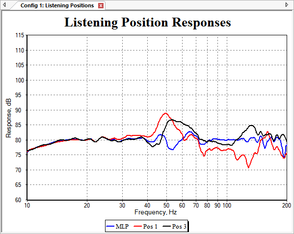
In order to choose the EQ level, we need to have MLP data that isn't contaminated with phase-related cancellation. This must be done using a "natural response" MLP plot, which mathematically forces all subs to be acoustically in phase with one another over all frequencies. In this way, it removes phase-related response dips that can't be compensated with EQ.

Explaining the EQ level is best done graphically as shown below.

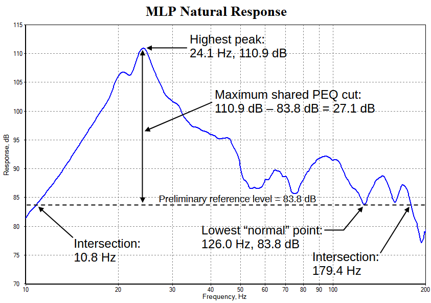
Picture using PEQs to equalize this response using only cuts and no boost. These PEQs will "squash" the response to either a fixed level or a prescribed target curve. In the case of a fixed level, this is the EQ level. The EQ level should be calculated as the deepest trough of the lowest "normal" response value as shown above.

Exercising Judgment When Determining the Lowest "Normal" Level

Some judgment is needed to determine what a "normal" level is when specifying it. In the graph above, we've chosen the lowest "normal" point to be at 126.0 Hz, where its value is 83.8 dB. Another reasonable choice would be the frequency of around 75 Hz, where the level of the dip is close to 86 dB. This would result in less loss of effective sub gain, at the expense of somewhat higher ripple of the final equalized response.

Two rules of thumb should be followed when choosing the lowest "normal" level.

• Don't use a frequency that's too high. In the plot above, if we were to use the dip at just below 200 Hz as the lowest "normal" level, we'd obtain an unreasonably low value. Subwoofer frequency responses, even MLP natural responses, tend to become chaotic above about 150 Hz in normal listening rooms. The higher the frequency at which you pick the lowest "normal" level, the more skepticism is in order.
• Likewise, don't use a frequency that's too low. A reasonable rule for determining what's too low is to never use the data at a dip whose frequency is below 20 Hz as the "normal" level. In typical listening rooms, the data below 20 Hz is strongly affected by the zero-order mode, which causes unpredictable behavior.

Determining the Maximum Allowable Shared PEQ Cut

With the EQ level chosen to be 83.8 dB, we can now figure out how much cut we'll allow for the shared sub PEQ filters. We can see from the graph above that at 24.1 Hz, the un-equalized response has a peak value of 110.9 dB. This means we need 27.1 dB of attenuation to knock the response down to 83.8 dB at that frequency. To simplify the discussion, we'll round this to 30 dB. This is quite a bit of attenuation. Will this have a bad effect on the system?

Having such a big un-equalized response peak at low frequencies turns out to help efforts to get low-distortion output rather than hinder them. The room mode is boosting the acoustical output in a frequency range where the subs would ordinarily struggle, taking the load off the amps and subs in that frequency region. Needing 30 dB of attenuation at 24 Hz means that, at that frequency, the amplifier power required to get 80 dB SPL is a factor of 1000 less than what would be needed if the un-equalized response were flat at 80 dB. That also means that the peak cone displacement needed to get 80 dB SPL is a factor of sqrt(1000) or 31.6x less than it would be if the un-equalized response were flat at 80 dB.

To properly take advantage of this situation, any large attenuation that we use must be provided by shared (input) PEQs as described in an earlier discussion, and not output PEQs. In this particular case, we're using the Flatten MLP response using only shared (input) filters optimization option, which disables output PEQs as part of the optimization itself. This means we're automatically covered in this example.

This large PEQ cut can have a disadvantage though. You might find that after applying the PEQ, the level of the subs is too low to match them up to the main speakers properly. In such a case, sub gains need to be turned up, and the subs re-measured before continuing with MSO. The automated room EQ of AVRs has an advantage over MSO in such a case, as such systems can give a "sub level too low" message early in the process. But MSO usage is a more manual process, so you'd do well to err on the side of sub gains being too high before measurement, rather than them being too low.

Determining The Optimization Frequency Range

The best way to figure out the optimization frequency range is to find the intersections of the horizontal line at the EQ level with the MLP natural response curve. To use this approach with the MLP curve shown above, press Ctrl+J to activate the graph's data cursor, and drag the cursor to the upper and lower frequencies where the curve reads 83.8 dB. Then press Ctrl+H to hide the data cursor. Using this technique, we obtain a lower limit of 10.8 Hz and an upper limit of 179.4 Hz. That's a good range if we want to be strict about it. But earlier in the examples, we were using 15 Hz and 190 Hz for some calculations. For consistency with earlier examples, we'll use 15 Hz to 190 Hz instead of the more rigorous 10.8 Hz to 179.4 Hz range.

Choosing the Reference Level for the Optimization Options Dialog

Paradoxically, the reference level you specify in the Optimization Options dialog is not critical at all. That's because MSO uses a shared sub gain block, which can shift the reference level (which is the final target level) to a wide range of convenient values. It is used as an optimization aid to getting the most accurate possible equalization, as described in detail in the topic titled The Shared Gain Block: A Special Kind of "Filter". After optimization, its value is discarded in the filter report. However, if you were to delete this gain block before optimizing, you would hamper MSO's ability to get the most accurate equalization possible. The reference level specified in the Optimization Options dialog would then become a kind of "magic reference level", which would need to be determined by multiple experiments. With a shared gain block present, this "magic level" is just an internal calculation that gets performed automatically by the optimizer, and you don't need to worry about it.

To make a long story short, we just pick the reference level for the Optimization Options dialog in a simple way. After determining the EQ level per the figure above, we just choose for the final reference level a position on the graph that's close to the EQ level. The EQ level in this case is 83.8 dB, so the final one could be 80 or 85 dB. We'll just pick 80 dB.

Although the reference level specified in the Optimization Options dialog is not critical, the EQ level is. That's because it's used in the computation of the maximum shared PEQ cut and the optimization start and stop frequencies as described above.

Setting The Optimization Options

Armed with the information we found above, we're ready to set all the optimization options.

Launch the Optimization Options property sheet as we've been doing.

Specifying the Optimization Type

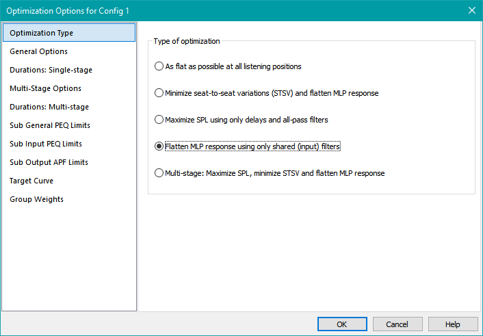
On the Optimization Type property page, choose the Flatten MLP response using only shared (input) filters optimization option as shown below.

Setting the General Options

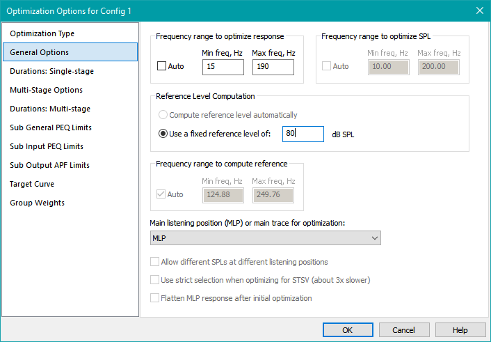
On the left side of the property sheet, choose General Options. Under Frequency range to optimize response, uncheck Auto and enter 15 for the lower frequency limit and 190 for the upper one. Next to Use a fixed reference level of:, enter 80 into the edit control.

You'll see that a number of options are disabled on this property page. UI controls are selectively enabled or disabled based on the optimization type chosen earlier on the Optimization Type property page. If a UI control is disabled, its contents are ignored for the optimization type you chose.

When done, the General Options page should look as below.

Specifying the Optimization Duration

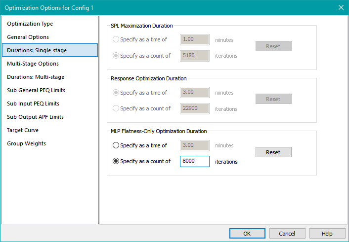
Select Durations: Single-stage on the left side of the property sheet. Only the controls in the MLP Flatness-Only Optimization Duration group should be enabled. Select the Specify as a count of radio button and enter 8000 into its edit control. The result should look as below.

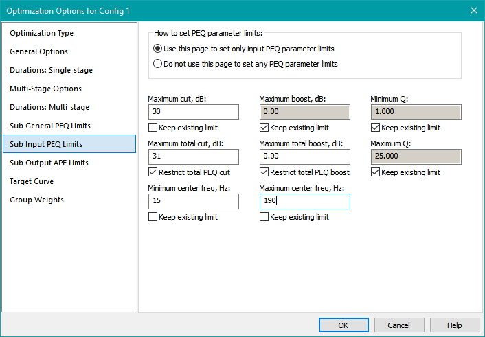
Setting the Input PEQ Parameter Limits

All that remains before optimizing is to set the PEQ parameter limits. We specifically want to set only the parameter limits of the input PEQs, as those are the only ones used for this type of optimization. The Sub General PEQ Limits contains a radio button that allows you to choose between setting the parameter limits for all PEQs (both input and output) or setting only the output PEQ parameter limits. Neither of these options is what we want, so we'll skip that page. Instead, choose the Sub Input PEQ Limits option on the left.

Make sure the Use this page to set only input PEQ parameter limits radio button is selected.

Earlier we determined that we needed to cut the response peak by 30 dB. Let's allow individual PEQs to have a 30 dB cut, while letting the cumulative cut (which can't be less than this) reach 31 dB. Under Maximum cut, dB, uncheck Keep existing limit and enter a value of 30. Under Maximum total cut, dB, enter a value of 31.

Best practice is to set the minimum and maximum PEQ center frequency limits to be the same as the minimum and maximum optimization frequencies respectively. Under Minimum center freq, Hz, uncheck Keep existing limit and enter 15 for this value. Under Maximum center freq, Hz, uncheck Keep existing limit and enter 190. All other controls can be kept as-is. When done, this property page should look as below.

Click OK to save the options. Before optimizing, make sure all the traces on the graph are visible using the technique described earlier.

Running The Optimization

Now we're ready to optimize the configuration. Right-click on the configuration in the Config View, then choose Optimize Configuration. When the optimization is complete, choose Yes when prompted to save the results, then save the project as user-guide-3.msop.

This is a somewhat disappointing result, both in terms of MLP flatness and STSV. Using the Performance Metrics dialog, we obtain the following results.

Errors after optimization with maximized SPL and flattened MLP:
SPL penalty: 1.84 dB
STSV: 1.98 dB
MLP target error: 1.01 dB

In the previous example where we optimized SPL only and captured the result in the file user-guide-2.msop, we got the following results.

Errors after SPL optimization:
SPL penalty: 1.84 dB
STSV: 1.98 dB
MLP target error: 18.99 dB

As the theory predicts, the SPL penalty and STSV did not change with the flattening of the MLP. These errors aren't affected by shared PEQs. As expected, the MLP target (flatness) error was greatly improved, from 18.99 dB to 1.01 dB.

Longtime users of MSO will notice that when the traditional method of optimization is used (Minimize seat-to-seat variations (STSV) and flatten MLP response), the STSV and MLP target error are usually much better than what's shown above. But the traditional method does not control for SPL penalty. An important thing to know is how much SPL we would give up by using that method. We'll try to get some insight into that question in the next section.