Optimization Example - Traditional Approach
What the Traditional Optimization Approach Does
Earlier examples demonstrated two different optimization approaches. These are called
- Maximize SPL using only delays and all-pass filters and
- Flatten MLP response using only shared (input) filters.
These names come from the Optimization Type property page of the Optimization Options property sheet.
These optimization types can be understood by the errors they try to minimize. These errors are all quantified in the Configuration Performance Metrics dialog. For SPL maximization, the error called Unweighted SPL penalty, dB is minimized. For flattening the MLP response (or forcing it to an imported target curve), the error called MLP target error, dB is minimized.
Another error listed in the Configuration Performance Metrics dialog is called Unweighted STSV error, dB. This is a measure of the seat-to-seat variation of the frequency responses. Our two previous examples don't incorporate this error into the optimization process. The example that follows uses an optimization type that incorporates both the seat-to-seat variation (STSV) and the MLP target error into what is optimized.
This is done by combining the two errors mathematically into a single error called Unweighted target/STSV error, dB. The optimization approach discussed next minimizes this combined error. This technique is the "traditional approach" that's been the staple of MSO for a number of years. In this example, we'll use the technique and show that it decreases the STSV and MLP target errors considerably over the previous two examples. We'll also find out its impact on the SPL penalty.
To minimize both the MLP target error and the STSV, both input and output PEQs are used. So for this example, we'll need to set the options for each group of PEQs on different property pages of the Optimization Options property sheet.
Preparing for the Optimization
Downloading the User Guide Examples: The data for this demonstration are available as getting_started_user_guide.zip. To get results that match the examples, please download and unzip this file before beginning if you haven't already.
Make a copy of the user-guide-3.msop and rename it to user-guide-4.msop. Open up this new project.
In addition, we want all the filter parameters in this optimization to start from a fresh state. To ensure this happens, choose Tools, Application Options from the main menu. Choose UI Options. This will show the property page below.
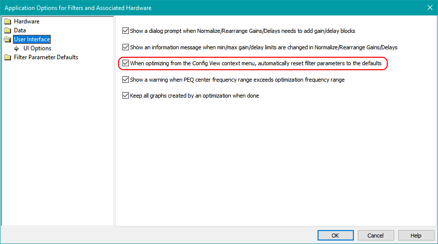
Make sure When optimizing from the Config View context menu, automatically reset parameters to the defaults is checked. Press OK when done.
Setting the Optimization Options
Right-click on the configuration in the Config View, then choose Optimization Options.
Specifying the Optimization Type
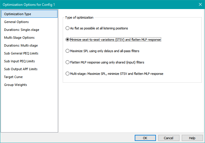
On the Optimization Type property page, choose Minimize seat-to-seat variations (STSV) and flatten MLP response. This property page should look as below.
Setting the General Options
Next, choose General Options. Since this project is based on the earlier user-guide-3.msop, the General Options page reflects the options we set in the previous optimization, in which we flattened the MLP response. These options are shown below.
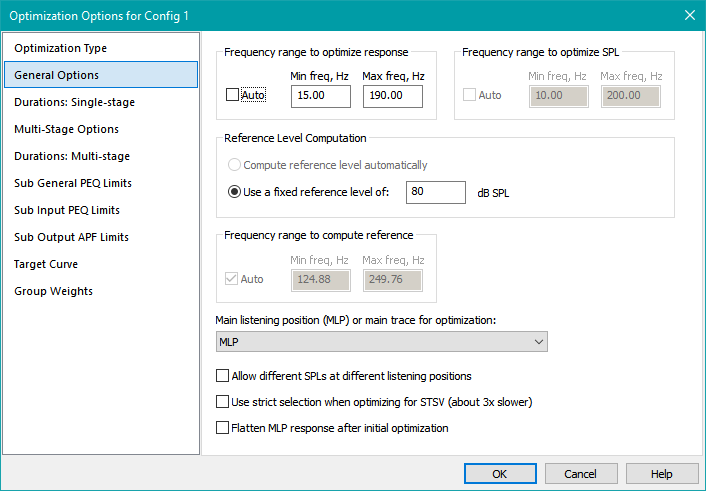
Since we'll be comparing the results of this optimization with the previous example, we can keep the frequency range of 15 Hz to 190 Hz the same. Likewise, the rationale for determining the reference level in the previous example remains valid, so we can keep that at 80 dB. No changes are therefore needed on this property page.
Specifying the Optimization Duration
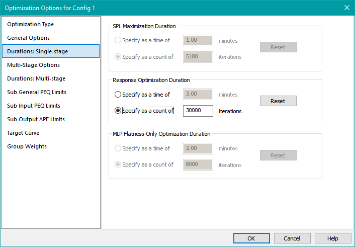
We can now move on to the Durations: Single-stage property page. Select Specify a count of and enter 30000 for the count of iterations. This property page should look as below.
Setting the Output PEQ Parameter Limits
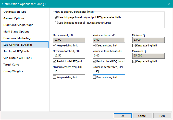
Next, select Sub General PEQ Limits. This is the property page used to set parameter limits for output PEQs. We were able to skip this page in the previous example because the Flatten MLP response using only shared (input) filters optimization type used in that example only requires input PEQs. But the Minimize seat-to-seat variations (STSV) and flatten MLP response we're using for this example makes use of both input and output PEQs. So we need to set their parameter limits.
On this property page, make sure the Use this page to set only output PEQ parameter limits radio button is selected.
In keeping with the previous guidelines about avoiding significant SPL degradation, we'll rely solely on the input PEQs to knock down the big 30 dB peak. However, in certain frequency bands, a sub may degrade the STSV due to room mode effects specific to that sub's location. Sometimes the only way to fix that is to knock down the level of that sub in the problematic frequency band. That band may be narrow enough that a high-Q PEQ may be able to do that without significantly degrading the overall SPL capability. Experience has shown that to knock an individual sub down enough to fix up the STSV may require a maximum PEQ cut of up to 12 dB. That's the default for this property page, so we'll keep it as-is.
Best practice is to set the minimum and maximum PEQ center frequency limits to be the same as the minimum and maximum optimization frequencies respectively. Under Minimum center freq, Hz, uncheck Keep existing limit and enter 15 for this value. Under Maximum center freq, Hz, uncheck Keep existing limit and enter 190. All other controls can be kept as-is. When done, this property page should look as below.
Specifying the Input PEQ Parameter Limits
Let's look at the Sub Input PEQ Limits property page now. In the previous example, we set it up for a maximum PEQ cut of 30 dB, with a cumulative PEQ cut limit of 31 dB. These EQ requirements haven't changed. They've carried over from the previous example, which is shown below.
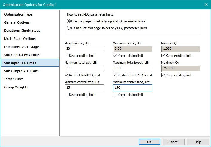
We can leave these options unchanged.
Specifying Output All-Pass Filter Parameter Limits
Choose Sub Output APF Limits on the left. That will show the associated property page as below.
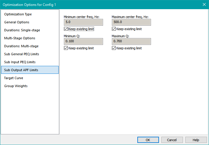
The parameter value limits for the all-pass filters can't be determined analytically. Instead, these limit values have been gathered from user experience.
Accept the default limits for the all-pass filter parameters and press OK to save all the optimization options.
Running The Optimization
Now we're ready to optimize the configuration. Right-click on the configuration in the Config View, then choose Optimize Configuration. When the optimization is complete, choose Yes when prompted to save the results, then save the project as user-guide-4.msop.
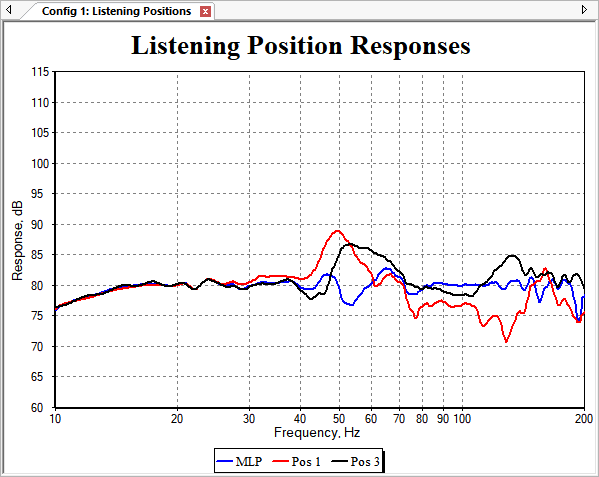
The result of the optimization is shown below. Optimization results vary somewhat from run to run, so this is a representative sample.
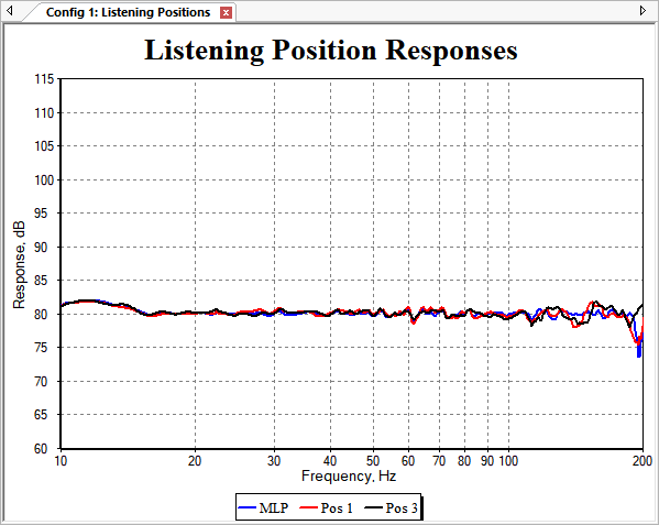
Visual inspection shows this to be a surprisingly good result for both MLP flatness and STSV. But what about the SPL penalty? Using the Performance Metrics dialog, we obtain the following results.
Errors after traditional optimization for STSV and MLP Flatness:
SPL penalty: 7.15 dB
STSV: 0.31 dB
MLP target error: 0.27 dB
Compare this to the previous optimization, in which the SPL was maximized, then the MLP flattened.
Here are the errors from the previous example as taken from the Performance Metrics dialog.
Errors after optimization with maximized SPL and flattened MLP:
SPL penalty: 1.84 dB
STSV: 1.98 dB
MLP target error: 1.01 dB
We've gotten big improvements in MLP flatness and STSV, but we've taken a 5.31 dB hit in SPL penalty (going from 1.84 dB to 7.15 dB). These examples are two extremes of performance emphasis, both of which are undesirable in some ways. This suggests that having the ability to trade off STSV and SPL penalty in a controlled way could give us a desirable middle ground with many of the advantages of both of these optimization types. We'll look at that possibility next.