Introduction to Optimization
A Word About the User Guide Optimization Examples
The details of the different optimization types can't be fully understood without concrete examples of their usage, along with practical tips to help ensure success. We'll build on the example project getting-started-2.msop from the Getting Started Guide to illustrate how to use the various optimization types. If you didn't go through that example, you can just download the files.
Each of the optimizations to be performed in the following sections use a separate project (.msop) file, with one configuration per project. Experienced users will note that there are advantages to putting all the different configurations in the same project. Using one configuration per project is just a way to avoid introducing the complexity of multiple MSO configurations too early in the discussion. This allows emphasizing the different optimization types without other distractions. Multiple configurations will be discussed later in the User Guide.
Some Preliminaries That Apply to All the Examples
Since the examples are all based on getting-started-2.msop project, let's have another look at the Configuration Properties page of the Configuration Wizard that was used to create the sole configuration in that project. This will tell us the types of filters we're using and how many of them there are.
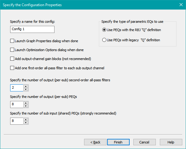
We can't actually go back through the wizard to see that page in the state it was originally filled out, so for now we have to rely on the screen capture of that state taken earlier. Later in this User Guide, we'll see how to find this information by inspection of the Config View, but we'll avoid such details for now.
We can see that we have the following filters in the project:
- No gain block in any output channel (checkbox is unchecked)
- No first-order all-pass filters (checkbox is unchecked)
- Two second-order all-pass filters per sub. In miniDSP devices, this means "two second-order all-pass filters in each output channel".
- Eight PEQs per sub (that is, eight PEQs in each output channel).
- Eight sub input PEQs (in other words, eight PEQs in the input channel)
Although there are no gain blocks in any output channel, MSO always puts a gain block on the input side. The purpose of this shared (input channel) gain block will be discussed in detail later, but we can say for now that the gain block allows flattening the MLP response to work as effectively as possible.
Avoiding Setups That Degrade SPL Capability
On the previous page, there's a section that addresses the new SPL maximization feature of MSO. In that section is the following statement.
"When the levels of one or more problematic subs are knocked way down compared to the others, the remaining subs have to work harder to get the same system SPL."
This is one of the keys to maximizing SPL. If you have identical subs, you want them all working equally hard so that as the subs approach their limits, no subs become over-stressed compared to any others. If your subs aren't identical, that adds more complexity that we'll delve into in Distortion Matching For Dissimilar Subs in the Tech Topics section. That procedure describes a technique for setting relative sub gains to obtain approximately equal distortion in all subs near their SPL limit. If you perform that procedure, all the methods and precautions we'll talk about in connection with SPL maximization will still apply.
Use Shared (Input) PEQs for Knocking Down Response Peaks
Suppose the frequency response of our combined subs in the absence of any EQ has one or more big peaks that need to be knocked down. What's the best way to do that? If we use the rule that all subs should be working equally hard to get the highest SPL capability, it follows that we should knock the responses of all subs down at once by the same amount. This is done with input PEQs (called "shared PEQs" in MSO).
The usage of shared PEQs in MSO is so important that it's required for two out of three of the new optimization methods introduced in MSO v2: Multi-stage: Maximize SPL, minimize STSV and flatten MLP response and Flatten MLP response using only shared (input) filters. Without them, MSO v2 doesn't offer that much additional capability over v1.
Use Output PEQs for Fighting Room Modes
Room modes don't just cause frequency response peaks and dips. They cause the responses at different listening positions to vary from one another to a surprising degree. One simplified way of thinking about this is by focusing in on a particular modal frequency. At that problem frequency, one or more subs might appear to "go rogue" in the sense that its phase response causes the problem sub to combine with the others in an undesirable way. Often an output PEQ, knocking down the response of just one or two subs in a narrow band of frequencies, can make the overall response in a neighborhood of that modal frequency flatter and with less seat-to-seat variation.
The project from the Getting Started Guide provides examples of both of these situations.
Use Graphs to Detect Undesired Phase Effects
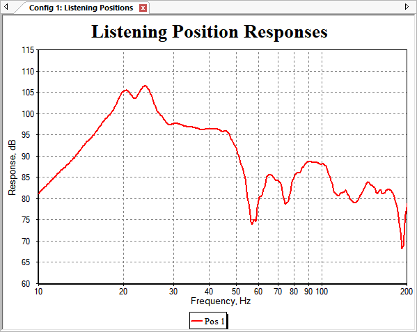
Let's have a look at how we ended up after finishing the Getting Started Guide.
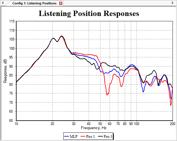
That response dip just below 60 Hz at the position Pos 1 looks suspicious. Could it be phase-related? Let's find out. First, we'll temporarily toggle all the graph traces off except for the suspicious Pos 1. Then we'll add a trace representing the so-called Natural Response of the system at the position Pos 1
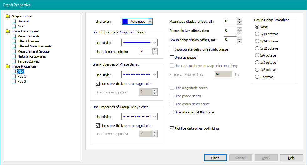
Both of these tasks can be done from the Graph Properties property sheet. Press Ctrl+G to launch it, then scroll down to the Trace Properties node and select the MLP trace. This will look as shown below.
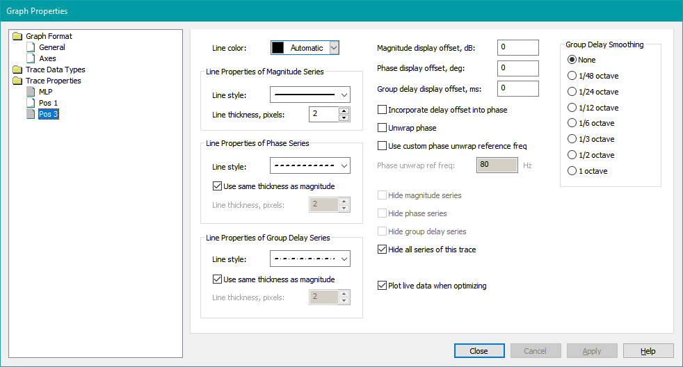
Since we're only interested in comparing the Natural Response of Pos 1 to the existing Pos 1 trace, we'll hide the MLP and Pos 3 traces. To do that, first check the Hide all series of this trace checkbox with the MLP trace node selected. Next, select the Pos 3 trace node and repeat this step. After doing this, the Graph Properties property sheet will look as below.
The icons representing the MLP and Pos 3 traces are now gray, indicating these traces are hidden. The graph will now look as below.
Now we need to add a Natural Response trace for Pos 1 to the graph. To do that, navigate to the Natural Responses node under Trace Data Types, check the checkbox next to Pos 1, then press Apply. The result will be as shown below.
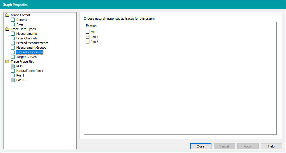
Notice that a new node representing the Natural Response trace for Pos 1 has been added under Trace Properties. If we wished, we could select the node and set the properties for this new trace. For now, we'll keep its default settings. The graph will now look as shown below.
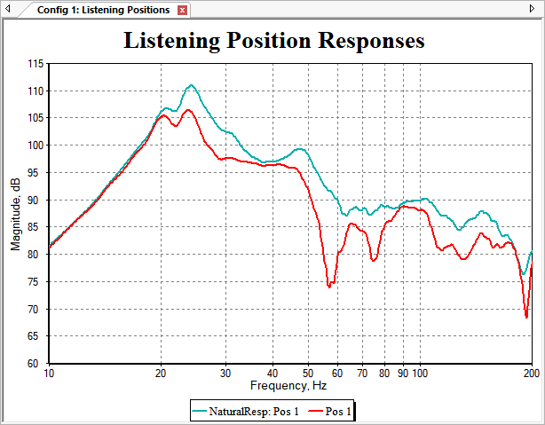
Press Close to close the Graph Properties property sheet. Now we can compare the "natural" and actual responses on the graph. Pressing Ctrl+J to activate the data cursor, then dragging it to the problem frequency gives the result below.
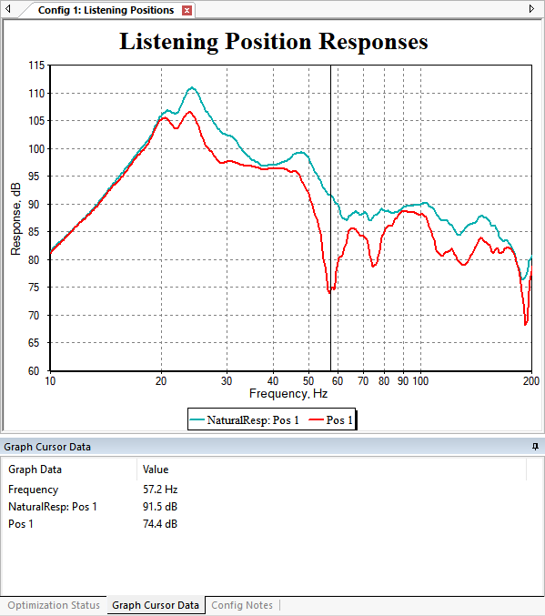
This shows that at 57.2 Hz, if all the subs were acoustically in phase with one another at Pos 1, we'd get 91.5 dB SPL output. But we're actually getting 74.4 dB SPL. So we're losing 17.1 dB at 57.2 Hz due to phase effects at Pos 1. There's no doubt that this is a phase-related dip. By examining the graph from the Getting Started Guide, it's also clear that this phase-related issue is the cause of the large seat-to-seat variation (STSV) at 57.2 Hz.
This raises an intriguing question. If we were to run a Maximize SPL using only delays and all-pass filters optimization, would the phase cleanup it performs also fix up the STSV, giving us the best of both worlds with respect to both STSV and SPL penalty? We'll look at this question in the next section. But first, we'll briefly look at another way to show and hide traces.
An Alternate Method for Toggling Trace Visibility
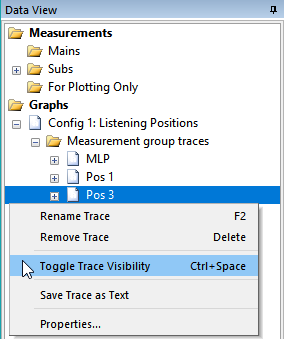
In addition to using the Graph Properties property sheet, you can also toggle trace visibility from the Data View. To do this, go to the Data View, expand the node for the graph so that the trace nodes are visible, then right-click on the trace you wish to hide and choose Toggle Trace Visibility. It's much faster to just select the trace node, then use the Ctrl+Space keyboard shortcut.
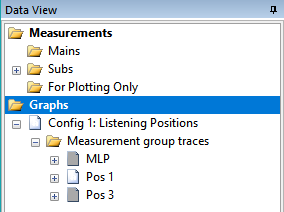
After doing that, the Data View will look like the image below. The hidden traces will have a dark gray icon.
We're Now Ready for the First Optimization
Now that we've finished some preliminary tasks and learned some techniques we can use for many optimization types, we're ready to do our first optimization.