The Details of Configurations
The Results So Far
In previous examples, we've performed the following steps:
- Used the Measurement Import Wizard to import the example measurement text files
- Used the Configuration Wizard to create a configuration
- Set the options of the graph created by the Configuration Wizard
-
Optimized the configuration in various ways
- Maximized SPL
- Flattened the MLP frequency response
- Used traditional MSO optimization to minimize STSV while flattening the MLP response
- Used the new composite optimization to minimize STSV and flatten the MLP response under the constraint that the SPL cannot be degraded by more than a set amount from the optimum.
- With those steps done, some measurement errors that can cause MSO's predicted response to differ from the actual final verification measurements were described.
- Specific techniques to avoid such errors in various scenarios were spelled out in detail.
Filling in Some Gaps
The different optimizations performed above were each done in a separate project (.msop) file. Experienced users going through those examples probably recognized that they could have all been done within a single project using multiple configurations. Avoiding discussion of multiple configurations at an early stage was just a way to avoid introducing too much complexity too soon.
We're now in a position to explore using MSO's more advanced capabilities. To make that possible, we first need to look at what configurations consist of, so we can make maximum use of them in later work.
Configurations in Detail
Configurations were first introduced in the Getting Started Guide. There, it was mentioned that one purpose of a configuration was to gather information about the DSP hardware: the number of channels, the type of filters to be used and how many of them there are, the filter parameter values, and so on.
With that in mind, we'll explore the connection between the block diagram of a popular DSP unit and the relevant portions of the structure of an MSO configuration as displayed in the Config View pane.
The Block Diagram of a Popular DSP Device
A DSP unit that can be used with MSO has a single input, hooked up to the subwoofer output of an AVR or preamp-processor (pre-pro). Processing begins with filters on its input. People generally refer to these as the "input filters". In MSO, they are also called the "shared sub filters". After the input signal is filtered, the resulting signal is passed along to (potentially) all the outputs through the matrix mixer. Each output has a bank of filters, a delay, and a gain adjustment among other things. Not surprisingly, people usually refer to the filters in the output channels as "output filters". In MSO, these are often called the "per-sub filters", as each DSP output channel is dedicated to a particular sub. To illustrate this, an annotated image of a block diagram of the signal processing of the very popular miniDSP 2x4 HD device is shown below.
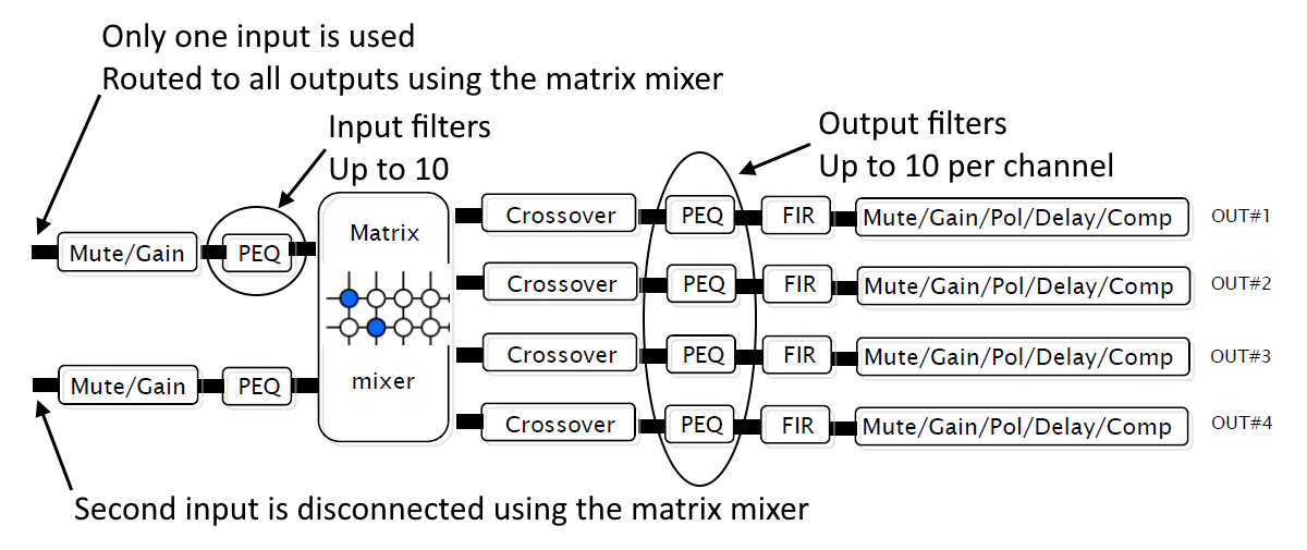
The original image was taken from the miniDSP 2x4 HD1 plugin datasheet PDF file.
The Anatomy of a Configuration
To see how a typical MSO configuration looks when expanded in the Config View, open up the user-guide-4.msop project. The Config View for this project is shown in the annotated diagram below. This diagram demonstrates the connection between the tree items in the Config View and the components of the DSP processor.
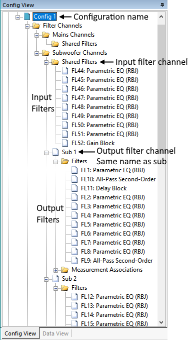
The topmost node of the configuration, labeled Configuration name above, is sometimes called the configuration's root node.
Filters and Filter Channels
Under each specific configuration node of the tree, such as Config 1 above, there is a collection of nodes under Filter Channels. These nodes are Mains Channels and Subwoofer Channels. We're interested in the Subwoofer Channels node and the ones under it. Under the Subwoofer Channels node, there is a Shared Filters node. Under the Shared Filters node is a collection of the input filters of the DSP device.
Try selecting one of these filters with the mouse, while observing the Properties Window (not shown above) on the right side of the MSO main window. This technique can be used to browse filter properties. It can also be used to modify them, but this is sometimes needed in certain special cases that we'll discuss soon. More will be said on the topic of filter properties shortly.
Also under Filter Channels for this project are four sub channels, of which only two are visible in the image above. In this case, the channels are named Sub 1, Sub 2, Sub 3 and Sub 4. They correspond exactly to the output channels in the DSP block diagram above. In MSO, there is only one Shared Filters node for the subs. It's always used as a container for sub DSP input filters if any. The number of sub output channels varies. They will be the same in number and have the same names that you gave the subs in the Configuration Wizard. When the Configuration Wizard is run, and you tell it the number of subwoofers and their names, it stores this information. Then, when it creates the configuration, it creates one channel for each sub, giving each channel the exact same name as the sub. That's how our channels ended up being named Sub 1, Sub 2, Sub 3 and Sub 4.
A shared gain block (FL52 in the image above) is always present, even if you choose not to have individual gain blocks in the Configuration Wizard. We'll talk more about its purpose shortly.
For sub-only configurations, there will be a delay block in all but one subwoofer channel. These maintain information regarding what DSP output channel delay should be for each sub, as shown in the DSP block diagram.
By comparing the annotations in the figure above with the annotations in the DSP block diagram, the relationship between the structure of the MSO configuration and the corresponding DSP device can be understood.
Configurations With No Shared Filters Are Strongly Discouraged
The filters in the Shared Filters folder node in the figure above correspond exactly to the input filters in the DSP block diagram. Configurations having no shared filters are now strongly discouraged in MSO since v2. MSO v2 adds three new optimization types to the two originally supported by MSO v1. Two of these additional three require that shared filters be present. These optimization types are listed below.
| Optimization Type | Needs Shared Filters |
|---|---|
| As flat as possible at all listening positions | No |
| Minimize seat-to-seat variations (STSV) and flatten MLP response | No |
| Maximize SPL using only delays and all-pass filters | No |
| Flatten MLP response using only shared (input) filters | Yes |
| Multi-stage: Maximize SPL, minimize STSV and flatten MLP response | Yes |
Optimization Types Requiring Shared Filters
If your configuration has no shared filters, when you launch the Optimization Options property sheet, you won't be able to choose either of the last two options above on the Optimization Type property page. This would prevent the most powerful new optimization type of MSO v2, Multi-stage: Maximize SPL, minimize STSV and flatten MLP response, from being used.
Working With Filters Manually
Sometimes the filters added by the Configuration Wizard might not fully meet your needs. In certain cases, you might want to modify your configuration without completely undoing previous work done to it. In such cases, you may need to add or remove filters manually. Adding filters manually allows you to use all filter types supported by MSO, not just those the Configuration Wizard supports.
We'll go into more detail shortly, describing some situations for which working with filters manually might be advantageous, and how to do it.
Before doing that, we'll take a brief detour into the subject of configuration measurement associations to complete our view of the structure of configurations. Then we'll return to the details of manual filter operations.
The Measurement Associations of a Channel
We can see that each individual channel (Sub 1, Sub 2, Sub 3 and Sub 4) has a Measurement Associations node underneath it in addition to the Filters nodes already discussed. If we collapse all the Filters nodes and expand the Measurement Associations nodes, we get the result shown in the annotated figure below.
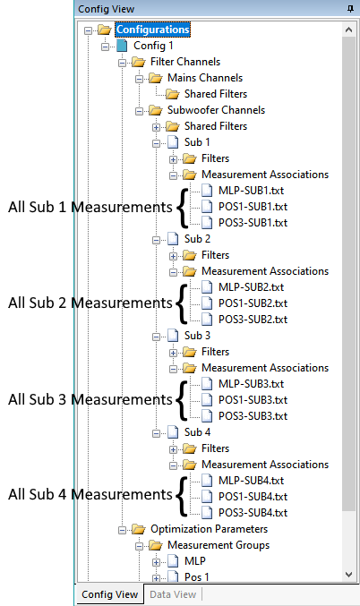
Here it can be seen that the measurement associations for the Sub 1 channel are all the measurements involving Sub 1, and likewise for the channels Sub 2, Sub 3 and Sub 4 and the respective measurements. The associations in this case mean that, as part of an intermediate MSO calculation, all the measurements for Sub 1 are modified in magnitude and phase by the response of the Sub 1 channel filters, with the same situation occurring for channels Sub 2, Sub 3 and Sub 4 and their respective measurements.
These associations are all set automatically by the Configuration Wizard.
Measurement Groups (Listening Positions) and Their Filtered Measurement Associations
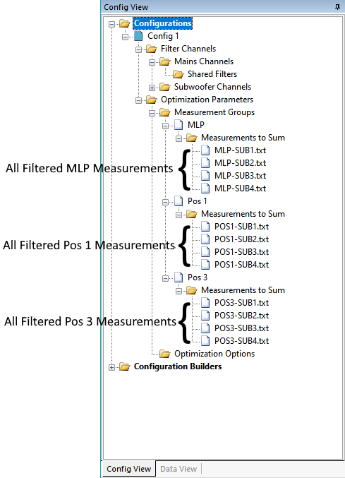
For typical MSO configurations, listening positions are called Measurement Groups. This name comes from the early days of MSO, which was originally written assuming people would use it to solve much more general problems than what the majority of people actually use it for nowadays. For all configurations created using the Configuration Wizard, a Measurement Group is the same thing as a listening position. Situations for which this is not the case are rare.
Measurement Groups can be thought of as being like a generalization of the A + B function of REW's Trace Arithmetic control in its All SPL view. But instead of calculating the sum of two measurements A and B, it calculates the sum of N terms at each listening position, where N is the number of subwoofers. Each term that's summed with the others is a sub measurement associated with that listening position, modified by the frequency response (both magnitude and phase) of the filter channel with which that sub measurement is associated. This is shown pictorially below. In this image, the number of filtered measurements listed under each Measurement Group is 4, which is the number of subs.
The Configuration Wizard takes care of setting up the messy details of all these measurement associations. Once you run the Configuration Wizard, there's no reason to change them. The purpose of these associations is to provide MSO with the information it needs to predict the frequency response (both magnitude and phase) at each listening position. That information is used for both static display of the response at each position, as well as during optimization, where these responses change as the optimizer adjusts filter parameters.
The Details of Filters
A good way to understand filter concepts in MSO is to start by understanding filter properties. As mentioned earlier, you can select a filter in the Config View on the left of the MSO main window, and its properties will be shown in the Properties window on the right. This is depicted below.
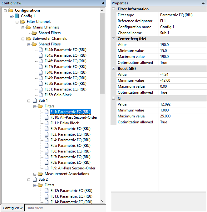
Filter Properties
Filter properties consist of two broad categories.
-
Filter Information contains a collection of text properties, each of which describes some attribute of the filter that can't be changed, such as:
- Filter type shows the type of filter, such as PEQ, low-pass, high-pass, low-shelf, high-shelf and so on.
- Reference designator uniquely identifies the filter, as you might see on a schematic diagram of an electronic circuit.
- Configuration name is the name of the configuration to which this filter belongs. This name is shown in the Config View. It is the configuration name you chose in the Configuration Wizard when creating the configuration.
- Channel name is the name of the channel that contains the filter. If this is a shared (input) filter, all the output channel names will be listed. This is because shared filters behave as if there is a separate copy of the filter in every output channel.
- A collection of filter parameters. Each filter parameter has a set of properties that we'll describe in more detail below.
As shown in the Filter Information, the selected filter FL1 shown above is of the Parametric EQ (RBJ) type. It belongs to the Sub 1 channel of the configuration Config 1. It has three parameters. They are called Center freq (Hz), Boost (dB), and Q.
Every filter parameter in MSO has four properties. It's useful to split these properties into three categories.
- The parameter value, defined by the property called Value. This is just the normal way we think of filter parameters. For the selected filter above, we can say, "The center frequency value of FL1 is 190.0 Hz".
- The parameter limits, defined by the Minimum value and the Maximum value. This is the range over which the optimizer is allowed to adjust the parameter's value. For this filter, we can say, "The optimizer is allowed to adjust the center frequency value of FL1 from 15.0 Hz 190.0 Hz".
- The Optimization allowed property of the parameter. This is a Boolean property (meaning it can be either True or False). The optimizer is permitted to vary the value of this parameter when Optimization allowed is True, and not permitted when it is False. In the image above, the optimizer is allowed to adjust all three parameter values.
So filter parameters are properties of filters, while the quantities listed above are properties of each parameter.
You can modify filter parameter property values by clicking in the right-hand column of the Properties window for the row of the property you wish to change. Then you can edit the value directly. If the cursor is currently in the left-hand column of the row, you can press F2 to jump to the right-hand column, which also selects its data for editing. After you change a property value in this way, its text will be highlighted in bold. In addition, the Value property has a spin-button control that allows you to tune the parameter value. If any displayed graph has traces that depend on the value of the parameter you're tuning, the traces will change in real time as you tune the parameter.
If a filter has multiple parameters, and you set the Optimization allowed property of one of them to False, the icon of the filter in the Config View will turn to a light gray color. If you set this property of all parameters to False, the filter icon will turn dark gray. If the filter has only one parameter, and you set its Optimization allowed property to False, the filter's icon will turn dark gray. The possibilities are summarized below.
- If the Optimization allowed property of all of a filter's parameters is True, the filter's icon will be white in color.
- If the Optimization allowed property of some, but not all of a filter's parameters is True, the filter's icon will be light gray in color.
- If the Optimization allowed property of all of a filter's parameters is False, the filter's icon will be dark gray in color.
- If a filter has no parameters at all, such as the polarity inversion element, its icon will always be dark gray in color because the optimizer cannot alter it.
Setting the Optimization allowed property of all the parameters of a filter to False, causing its icon to be turned dark gray, means that filter's parameter values will not be altered in any way by the optimizer. This is known as filter locking. Setting the Optimization allowed property of all the parameters of a filter to True, making all parameters optimizable, is known as filter unlocking. When these operations are done on a single filter parameter, they are referred to as filter parameter locking and filter parameter unlocking respectively. These operations on filters will be discussed in detail below.
Modifying Filter Parameters in the User Interface
The properties of filter parameters can be modified in the user interface in multiple ways. These include:
-
Modifying filter parameter limits.
- You can modify filter parameter limits on an individual filter basis using the editing technique described above for the Properties window.
- Filter parameter limits can be modified for multiple input PEQs, output PEQs and output all-pass filters at once using the Sub Input PEQ Limits, Sub General PEQ Limits, and Sub Output APF Limits property pages respectively of the Optimization Options property sheet.
-
Modifying filter parameter values.
- In the Properties window, you can modify parameter values of individual filters using the editing technique described above. This includes tuning the values by using the spin button control that appears when you click in the right-hand column of a parameter's Value property.
-
Modifying parameter values of many filters in a configuration at once can only be done by resetting all the parameters of the configuration to their defaults.
- This is done by right-clicking on the configuration's root node and choosing Reset All Filter Parameter Values. This sets the values of all unlocked filter parameters to their defaults, but leaves the values of all locked parameters intact.
- The default values of all parameters of all filter types can be specified in the Filter Parameter Defaults property pages of the Application Options property sheet by choosing Tools, Application Options, Filter Parameter Defaults from the main menu.
-
Locking and unlocking filters.
- To lock all the parameters of a filter, select the filter in the Config View. Right-click and choose Lock Filter Parameters from the context menu. If the parameters are already locked, you can unlock them with the context menu's Unlock Filter Parameters command.
- These locking and unlocking commands are available at many levels in the tree of the Config View. This means you can lock or unlock many filters at once. For instance, you could lock all shared sub filters of a configuration by right-clicking on the Shared Filters node under Subwoofer Channels and choosing Lock Shared Sub Filter Parameters.
-
You can combine these commands in various ways to make locking and unlocking of filters quicker. For instance, if you wanted to lock all shared sub filters except one, you could do the following:
- Use the command described just above to lock all shared sub filters.
- Right-click on the shared sub filter you wish to unlock, and choose Unlock Filter Parameters from the context menu. This approach is much quicker than locking many filters one at a time. We'll illustrate this technique later in a real-world example.
Adding and Removing Filters Manually
For all the examples we've looked at so far, all the filters of the configurations we've optimized were created and added by the Configuration Wizard. But there may be some cases for which we want to add or remove filters to achieve a specific objective.
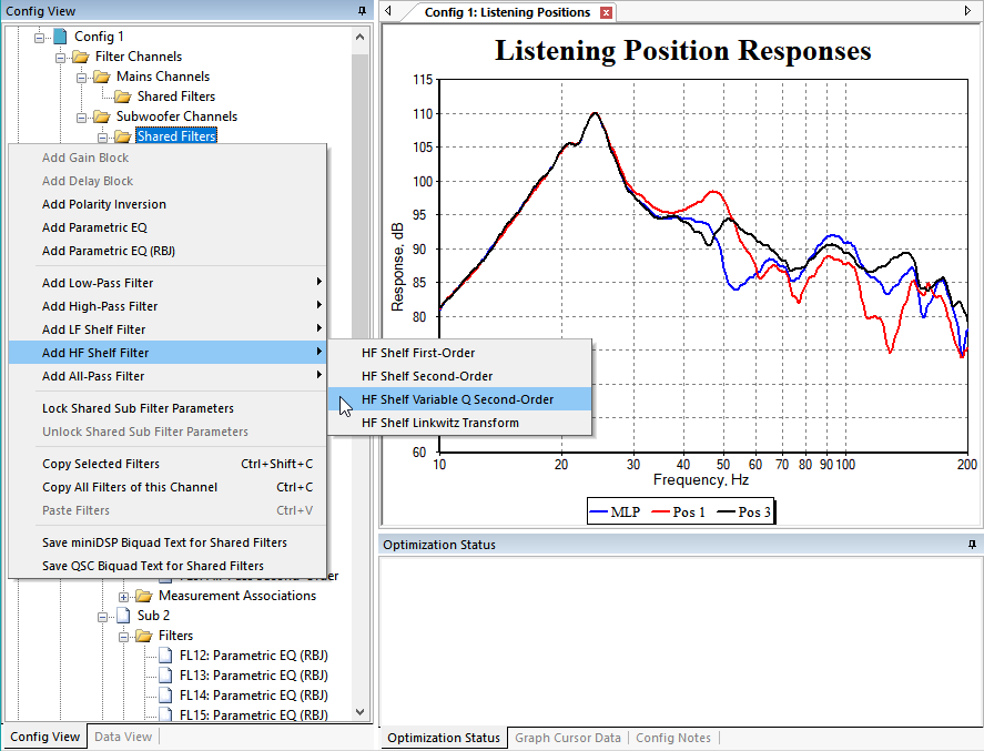
One such case arises when trying to fix a high-frequency roll-off problem like what we discussed earlier. Many methods to eliminate such high-frequency roll-off in the measurements were discussed. If you've tried all of those methods and there's still some high-frequency roll-off that you can't get rid of (like a sub amp with a low-pass filter that can't be defeated), you can counteract that effect if it's not too extreme by adding a high-shelf filter to the shared sub channel in MSO. Below is an illustration of how that might be done.
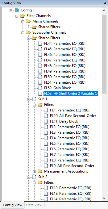
After adding the filter, it shows up under the Shared Filters node of Subwoofer Channels as shown below.
In an earlier section, we illustrated on a graph how an unwanted sub LPF could cause problems for the high-frequency response. That illustration was made with the help of the technique shown above for adding filters manually. In that case, an LR4 LPF at 120 Hz was added to the shared sub channel.
Later we'll look at specifics of how to use a shelving filter to get rid of the high-frequency roll-off that exists in this example.
To delete a filter, just select it and press the Delete key. If you accidentally delete a filter, you can add one back in using the technique described above for adding filters. When you do that, the added filter will have default values for its parameter limits as determined by the associated Filter Parameter Defaults property page of the of the Application Options property sheet. You'll need to set those limits to match the other filters, which is easiest from the appropriate property page of the Optimization Options property sheet.
The Shared Gain Block: A Special Kind of "Filter"
All of the MSO signal processing blocks are called "filters", even though some of them, like gain blocks, delay blocks and inverters aren't really filters at all. This is just to give them a name that isn't too cumbersome. We'll just call them "gain blocks" here.
The discussion below only applies to sub-only configurations and the effect of the gain block on equalization. For subs+mains configurations, this gain block represents the change in AVR sub trim that needs to be made. We won't discuss that further here.
A shared gain block is always added to a configuration by the Configuration Wizard even if the wizard's Add gain blocks (not recommended) option on its last page is unchecked (as it should be in the vast majority of cases). This is because it serves an important function when performing equalization.
Conventional equalization is new in MSO v2. It's used with the Flatten MLP response using only shared (input) filters optimization option. We'll use that feature in the next topic to flatten out some unwanted high-frequency roll-off.
This shared gain block isn't different from any other gain block in any way. But given its location in the shared sub gain path, it serves an important function that may not be obvious at first glance. To understand this importance, we'll take a slight detour to look at equalization in REW. The reason for this should become clear in a moment.
Here's an image of some un-equalized REW data, along with a target curve.
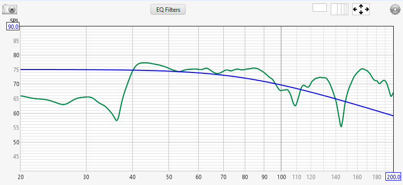
If all we can do with equalization is to cut the response, we could only bring the parts of the measured response that are above the target down to the target. This is shown below.
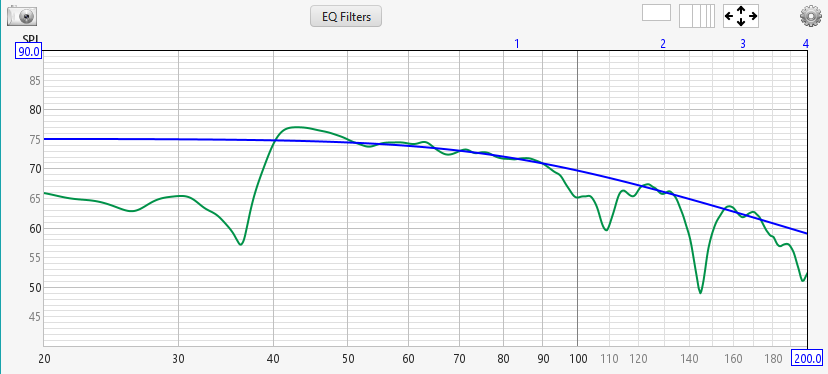
This equalization run couldn't to do anything with those parts of the curve already below the target.
Suppose we raised the target curve so that all of it is above the data as shown below.
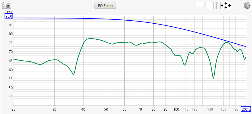
In this case, with only attenuation available to match the measurement to the target, we wouldn't be able to get any result at all, because the data is already below the target at all frequencies. Here, our target curve is too high.
Now suppose the maximum allowable cut in our equalization were, say, 10 dB. If we were to put the target curve way below the measured data, we might get something like the image below.
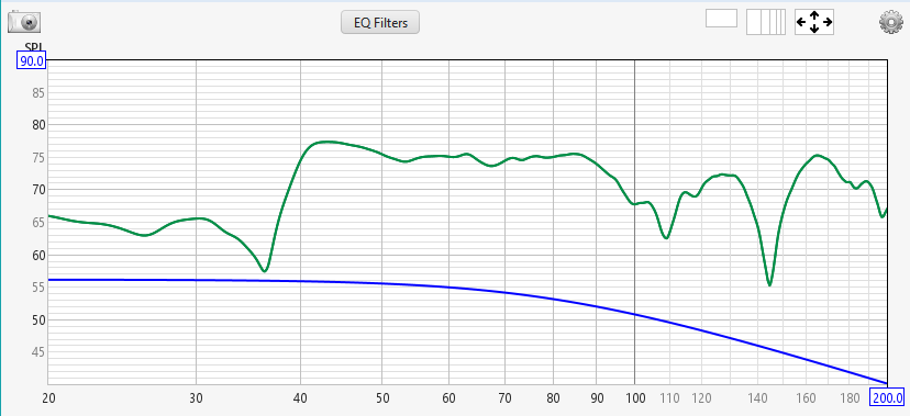
With a maximum allowable cut of 10 dB, we won't always be able to cut enough from the measured data to reach the target. In the frequency range from 40 Hz to 100 Hz for instance, the measured data is more than 10 dB above the target, so 10 dB is not enough cut to shift the measurement data to the target. The target curve is too low.
Once we set a maximum allowable cut in the equalization, then somewhere between the two extremes of "too high" and "too low" above, there is some optimum level for the target curve that would give us the best possible fit between the equalized data and the target after the equalization is performed.
It would be nice if the equalization or optimization software would automatically adjust this target level for us, so that we could always achieve a result as close as possible to the optimum. That's what the shared gain block in MSO does. Only instead of having a variable target that adjusts itself up and down, the shared gain block adjusts the gain of the subwoofers all at once, shifting the equalized response curves up or down relative to the fixed target. This accomplishes the same thing as having a variable target that automatically shifts itself up or down. Given a fixed value of the maximum allowable cut in the equalization, this gain shifting allows us to make the best use of the allowed equalization range of the filters to achieve the best possible fit between equalized curve and target. Using it is the equivalent of finding the optimum target curve level in the examples above automatically. That's why you should always have a shared gain block.
Revisiting the Reference Level
Please note that the reference level in MSO has nothing whatsoever to do with AVR reference levels.
Let's briefly go back to some earlier optimizations we did. After first optimizing for maximum SPL, which does not require a reference level to be specified, we went on to optimize the MLP flatness. To do that, we first found the EQ level and the reference level as described in an earlier topic. We did that by looking at a graph of the MLP natural response. That graph is repeated below.
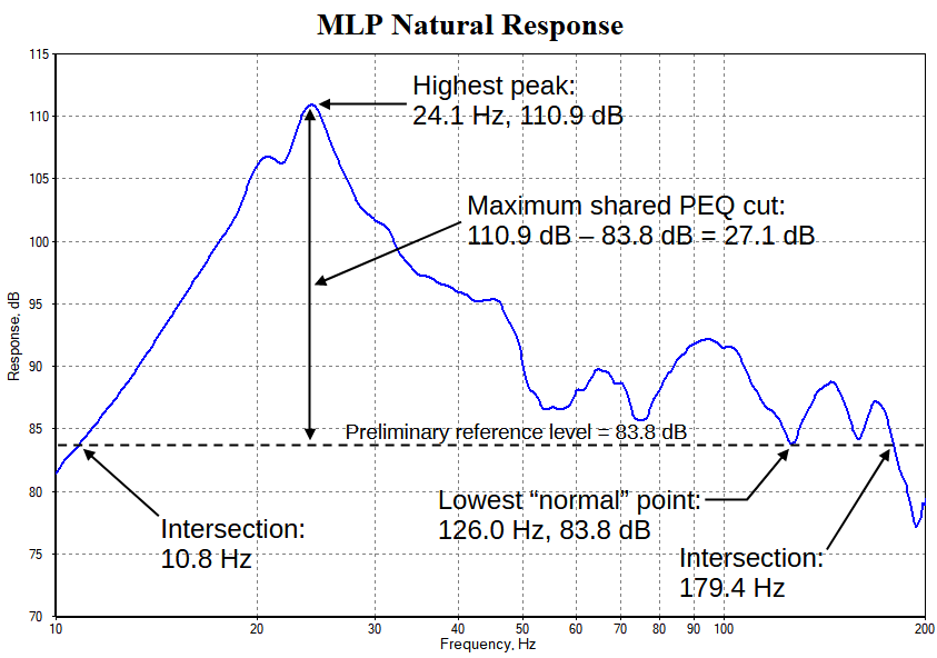
We looked at the depths of the response troughs to find a level we could achieve using only equalization cuts. In the image above, we can see that if we choose the level at 126 Hz of 83.8 dB, we can reach that level using only cuts all the way up to 179.4 Hz. We called this the EQ level.
Using the EQ level, we looked at the response peak, which reaches 110.9 dB at around 24.1 Hz. We then calculated that the input PEQ filters needed to have a maximum cut of 27.1 dB, so the peak response value of 110.9 dB could be brought down to 83.8 dB to make the response flat.
Thus the EQ level, combined with the response value at the highest peak, determines what our maximum allowable cut needs to be for the input PEQ filters. We must then enter that maximum cut in the Sub Input PEQ Limits property page of the Optimization Options property sheet.
The next step in our previous optimization was to flatten the MLP response. One of the things we needed to do before performing that operation was to specify the reference level on the General Options property page of the Optimization Options property sheet. That's shown below.
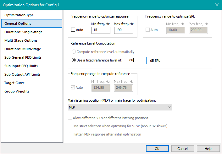
Does the reference level need to be the same as the EQ level? The answer to this question is "no". Recall the observation above in the discussion regarding REW equalization.
"Once we set a maximum allowable cut in the equalization, then somewhere between the two extremes of "too high" and "too low" above, there is some optimum level for the target curve that would give us the best possible fit between the equalized data and the target after the equalization is performed."
This maximum allowable input PEQ cut was determined using the EQ level. It is therefore the EQ level, not the reference level, that matters to the optimization. With a shared gain block (as in MSO), the adjustment of its gain value to shift the equalized response up and down relative to a fixed target has the same effect as shifting the target relative to a response of a system whose gain is fixed (as in the REW examples above). We can say that, provided the shared gain block has enough adjustment range, the reference level can be considered to be purely cosmetic. The Configuration Wizard always adds a shared gain block with an allowable range of 0±24 dB, so it should always have plenty of adjustment range to accommodate any reasonable reference level.
Once we find the maximum PEQ cut per the graph above, We would then enter that value into the Sub Input PEQ Limits property page of the Optimization Options property sheet. What should the reference level on the General Options property page be in this case? We could make it 83.8 dB if we wanted, but that isn't necessary. If we choose an 80 dB reference level instead, assuming our graph has the standard 5 dB/div on the vertical axis, the equalized trace on the graph will end up being lined up with a horizontal grid line on the graph. Ideally, the only difference between a reference level of 80 dB and 83.8 dB would be a different gain value for the shared gain block. The decision with all the impact here was choosing the EQ level to be 83.8 dB, not choosing the reference level to be 80 dB.
Next Steps
In the next section, we'll use these ideas to add a high-shelf filter that equalizes the high-frequency roll-off of this system.