Optimization Example - Composite Method

Summarizing What We've Done So Far

In the previous three examples, we've done the following:

• Run a Maximize SPL using only delays and all-pass filters optimization without trying to flatten the response at the MLP.
  • This gave us a low SPL penalty of 1.84 dB.
  • The MLP target error was very high at 18.99 dB because we did not try to flatten the MLP response.
• Run a Flatten MLP response using only shared (input) filters to clean up the MLP response.
  • This retained the low SPL penalty of 1.84 dB from the previous optimization.
  • The MLP target error was greatly reduced, from 18.99 dB in the previous optimization to 1.01 dB.
  • The seat-to-seat variation (STSV) ended up as 1.98 dB. Looking at a plot of the final result shows much room for improvement, both in the MLP target error and STSV.
• Run a traditional Minimize seat-to-seat variations (STSV) and flatten MLP response optimization.
  • This resulted in excellent STSV and MLP target error.
    • The STSV value was 0.31 dB.
    • The MLP target error was 0.27 dB.
    • Looking at a plot of the optimized result shows almost no room for improvement of either the STSV or MLP target errors.
  • The SPL penalty was degraded.
    • The SPL penalty increased from its prior value of 1.84 dB to 7.15 dB
    • This SPL penalty is a degradation of 5.31 dB relative to our SPL-optimized value.

These results can be summarized more simply as follows.

• If our optimization only minimizes SPL penalty and flattens the MLP, the STSV and MLP target error end up being too high.
• If we optimize STSV and MLP target error without taking the SPL penalty into account, the SPL penalty ends up being too high.

Controlling the Trade-Off Between STSV and SPL Penalty

Given the results so far, it's reasonable to conclude that what's needed is a way to trade off seat-to-seat variation (STSV) error and SPL penalty. Our hope is that by making a small concession in the form of an SPL penalty that's slightly higher than the optimum, we might get an outsized improvement in the STSV and MLP target errors.

That is the problem the Multi-stage: Maximize SPL, minimize STSV and flatten MLP response optimization method was intended to solve. In this example, we'll use the technique in an effort to obtain a result with a desirable trade-off between STSV and SPL penalty.

Multi-Stage Optimization

The Multi-stage: Maximize SPL, minimize STSV and flatten MLP response optimization method uses a new feature of MSO v2: multi-stage optimization. It's best understood by comparing it with the original MSO approach of using only a single stage of optimization.

In single-stage optimization, the following steps are performed.

• A copy of the configuration to be optimized is made.
• An optimization is run on this copy.
• At the end of the optimization is a prompt dialog asking you if you want to retain the optimized result.
  • If you choose "No", the optimized configuration copy is discarded.
  • If you choose "Yes", the optimized configuration copy overwrites the original.

The new Multi-stage: Maximize SPL, minimize STSV and flatten MLP response optimization method performs the following steps.

• Before the optimization begins, a copy of the configuration to be optimized is made.
• The first optimization stage does the equivalent of the Maximize SPL using only delays and all-pass filters method we performed earlier. This is done on the copy of the configuration made above. This stage does the following.
  • All PEQs are forced to a flat response condition and their parameters locked so the optimizer can't change them.
  • All parameters of all filters except delays and all-pass filters are locked.
  • An optimization is run to minimize the SPL penalty by changing only the parameters of delays and all-pass filters.
  • After this optimization completes, all filters that had their parameters locked are unlocked again so that subsequent optimization stages can modify them.
  • This modified configuration is passed on to the next stage of optimization, along with the value computed for the final SPL penalty.
• The second stage of optimization receives the configuration as modified by the first stage above. It performs an optimization very similar to the single-stage method called Minimize seat-to-seat variations (STSV) and flatten MLP response, but with several twists.
  • The delay and all-pass filter parameters have user-supplied limits applied to them to prevent these parameter values from straying too far from the ones that maximized SPL in the first optimization stage.
    • These limits are a restricted subset of the ones specified in the Optimization Options dialog and are never used to make the previously specified limits wider.
  • The same global constraint system that prevents PEQ "stacking" also prevents the SPL penalty from exceeding a limit that depends on the optimum value passed on from the first stage of optimization. We'll see how to specify that limit shortly.
  • A technique called multi-objective optimization (named "strict selection" in the Optimization Options) can be optionally used in this stage. Though slower than the conventional optimization approach, it is sometimes able to find solutions that the traditional approach isn't able to find.
  • After this stage of optimization completes, the filter parameter limits are reset to the values specified in the Optimization Options and the modified configuration is passed along to the third optimization stage.
• The third and final stage of optimization receives the modified configuration from the previous stage. It then performs the following tasks.
  • It locks all parameters of all filters except the shared sub filters.
  • It resets the parameters of all shared sub filters to their defaults so it can start its task from scratch.
  • It flattens the MLP response.
  • After flattening the MLP response, it unlocks all the filter parameters it locked in the first step.
• At the end of the final optimization stage, a prompt dialog asks you if you want to retain the optimized result.
  • If you choose "No", the optimized configuration copy is discarded.
  • If you choose "Yes", the optimized configuration copy overwrites the original.

This is a complex sequence of steps, but it's not difficult to give MSO the information it needs to perform them. We'll do that next.

Preparing for the Optimization

Downloading the User Guide Examples: The data for this demonstration are available as getting_started_user_guide.zip. To get results that match the examples, please download and unzip this file before beginning if you haven't already.

Make a copy of the user-guide-4.msop from the previous example and rename it to user-guide-5.msop. Open up this new project.

Setting the Optimization Options

Right-click on the configuration in the Config View, then choose Optimization Options.

Specifying the Optimization Type

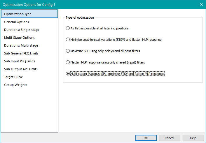
On the Optimization Type property page, choose Multi-stage: Maximize SPL, minimize STSV and flatten MLP response. This property page should look as below.

Setting the General Options

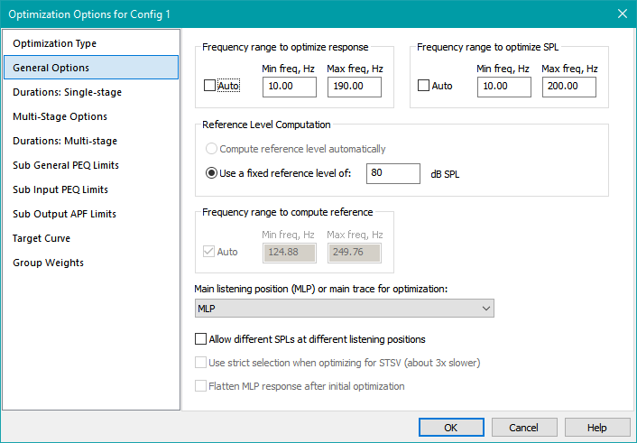
Next, choose General Options. Under Frequency range to optimize response, make sure Auto is unchecked and set the range to be 10 Hz to 190 Hz. The reduction from 15 Hz to 10 Hz of the minimum frequency for response optimization reflects some previous work we did using the MLP natural response to set the reference level.

Under Frequency range to optimize SPL, make sure Auto is unchecked and set the range to be 10 Hz to 200 Hz. Also, make sure the reference level is set to 80 dB. The result should look as below.

Some Property Pages Are Disabled

If you try to set the optimization durations using the Durations: Single-stage property page, you'll see all the controls on the page are disabled. That property page is not applicable to multi-stage optimization, so MSO disables those controls in this case. In general, you'll see that depending on the type of optimization you choose on the Optimization Type property page, different controls on different property pages may be disabled. That's to simplify data entry by disabling controls that have no effect for the chosen optimization type.

Specifying the Multi-Stage Options

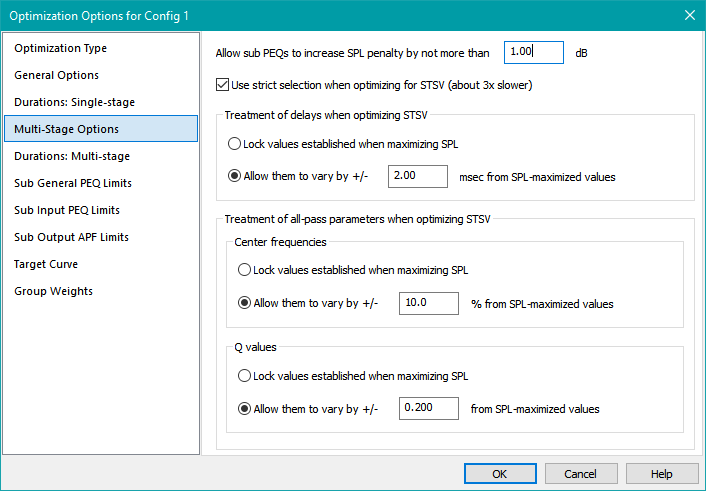
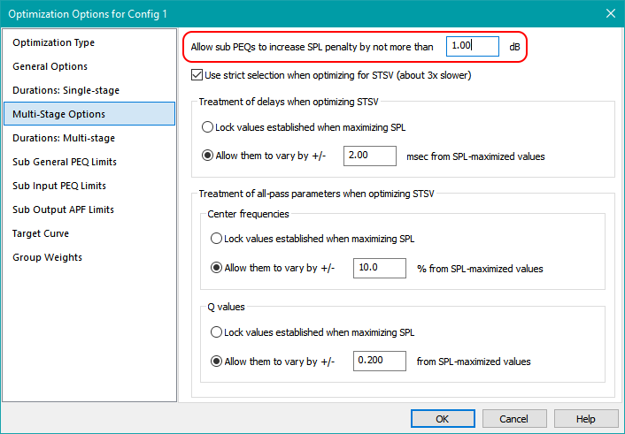
Select the Multi-Stage Options property page and set the various options as shown below.

The options shown above require some explanation. These options pertain to the second stage of the multi-stage optimization and assume that the first stage has already been performed.

The first optimization stage determines the lowest SPL penalty that can be practically achieved with the given choice of all-pass filters and delays and their allowed parameter ranges. Suppose for the sake of argument that in this first stage, the best SPL penalty achievable was calculated to be 1.8 dB. This value is passed on to the second optimization stage. That's where the value of the Allow sub PEQs to increase SPL penalty by not more than option shown above comes in. That value in the settings above is 1.0 dB. This means that in the hypothetical situation of a best-case SPL penalty of 1.8 dB, the allowable SPL penalty when optimizing for STSV in the second stage will be 2.8 dB (= 1.8 dB + 1.0 dB). All potential solutions having an SPL penalty greater than 2.8 dB will be rejected in the second optimization stage in this hypothetical situation.

The Use strict selection when optimizing for STSV option enables an optimization technique called multi-objective optimization. The details of this approach are too complex to get into here, but in short, the technique can sometimes find better solutions at the expense of requiring longer to complete. For this example, we'll enable it.

Next are three groups of options that all have a related purpose: that of allowing to some extent the emulation of some of the manual approaches that have been used for SPL maximization with earlier MSO versions.

One example of this manual approach uses delays and all-pass filters to maximize SPL, then locks all the delay and all-pass filter parameter values prior to running an additional optimization to minimize the STSV and flatten the MLP response. The equivalent of such an approach using the options above would be to choose Lock values established when maximizing SPL in all three groups of options.

To provide additional flexibility, the Multi-Stage Options property page allows you to specify that the delay and all-pass filter parameter values found in the initial SPL maximization phase are to each be used as the center of an allowable range. Doing so can help optimizer convergence by suitably restricting the ranges of these critical parameters, while also allowing some adjustment to achieve the best possible STSV for the allowed SPL penalty.

In the above example, allowed deviations from previously optimized parameter values are ±2.0 msec for delays, ±10.0% for all-pass center frequencies and ±0.2 for all-pass Q. MSO automatically constrains these limits to be within the values you specify on the Sub Output APF Limits property page. We'll use the options shown above in this example's optimization.

Setting the Optimization Durations

Select the Durations: Multi-stage property page. Enter the option values shown below.

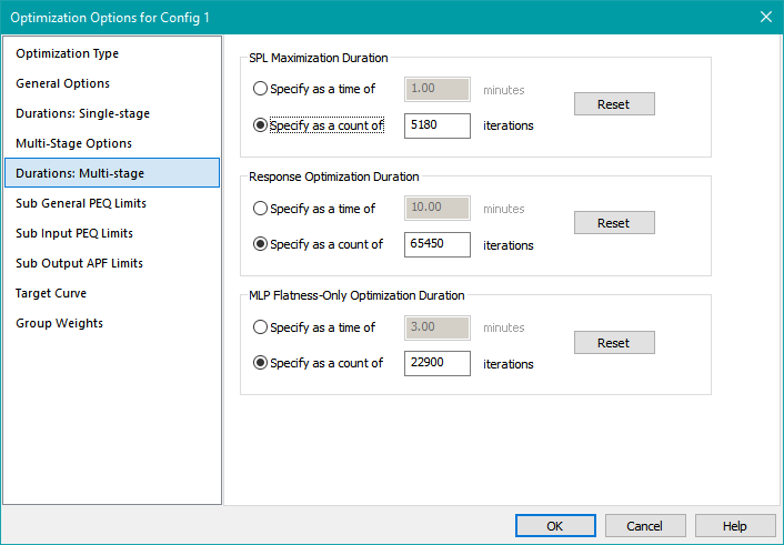
This property page is used exclusively for the multi-stage optimization method. Since the method has three stages and each stage's complexity is different, each stage must have an optimization duration specified separately for it.

Best practice for MSO v2 is to specify optimization duration in terms of a count of iterations rather than specifying a time. Reasons for this recommendation include:

• Once a suitable count of iterations is specified, results of similar quality will be obtained regardless of the speed of the machine used, the number of concurrent threads it supports and so on.
• In forum troubleshooting, insufficient or excessive optimization duration can be identified if the duration is specified as an iteration count. The iteration count provides a common frame of reference allowing meaningful comparison across many user systems.
• Even for a given machine, the number of iterations that can be performed in a given time depends on what else the machine is doing. Playing video might slow the machine down. Even web browsing can have a significant effect, as many web browsers aggressively create a large number of execution threads as more web pages are opened.

If you need to find a reasonable starting point for the number of iterations to use, use the Reset button for the particular duration you wish to set. This will replace the value you entered with its default for the given optimization type. Repeat for all three optimization stages as needed. The above values were determined in this way.

Setting the Output PEQ Parameter Limits

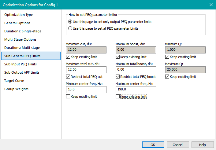
Select Sub General PEQ Limits. As in the previous example, this is the property page used to set parameter limits for output PEQs. On this property page, make sure the Use this page to set only output PEQ parameter limits radio button is selected.

As we did in the previous example, we'll follow the earlier guidelines about avoiding significant SPL degradation. For instance, we'll rely solely on the input PEQs to knock down the big 30 dB peak. For the output-side PEQs, we'll follow the approach from the traditional optimization example. That means we'll just use the default for this property page. The maximum individual PEQ cut of 12 dB here might seem high, but the SPL penalty is constrained in this optimization stage, so that prevents undesired SPL degradation. Experience with this example has shown that a 12 dB allowable cut gives better STSV results for a given allowable SPL penalty than e.g. 6 dB. That is a counter-intuitive result.

As before, we'll use best practices for the minimum and maximum PEQ center frequency limits, setting them to be the same as the minimum and maximum optimization frequencies respectively. Earlier, we set the minimum response optimization frequency to 10 Hz. So under Minimum center freq, Hz, uncheck Keep existing limit and enter 10 for this value. Under Maximum center freq, Hz, uncheck Keep existing limit and enter 190. All other controls can be kept as-is. When done, this property page should look as below.

Specifying the Input PEQ Parameter Limits

Select the Sub Input PEQ Limits property page. In the prior example, we set it up for a maximum PEQ cut of 30 dB, with a cumulative PEQ cut limit of 31 dB. Those EQ requirements haven't changed. They've carried over from the original MLP response flatness example. However, we've decreased the minimum response optimization frequency from 15 Hz to 10 Hz. Because of this change, under Minimum center freq, Hz, we need to uncheck Keep existing limit and enter 10 for this value.

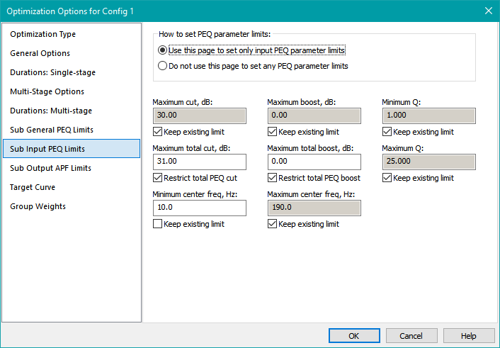
We can leave the rest of the options unchanged.

Specifying Output All-Pass Filter Parameter Limits

Choose Sub Output APF Limits on the left. That will show the associated property page as below.

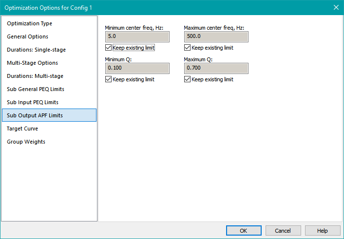
As in previous examples, the parameter value limits for the all-pass filters can't be determined analytically. Instead, these limit values result from user experience.

Accept the default limits for the all-pass filter parameters and press OK to save all the optimization options.

Running The Optimization

Now we have all the information we need to optimize the configuration. Right-click on the configuration in the Config View, then choose Optimize Configuration. When the optimization is complete, choose Yes when prompted to save the results, then save the project as user-guide-5.msop.

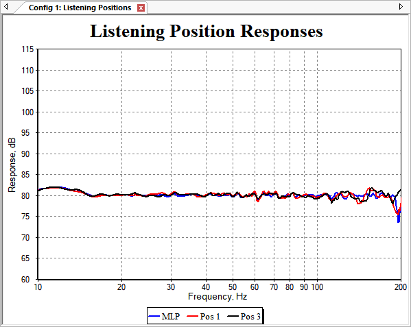
The result of the optimization is shown below.

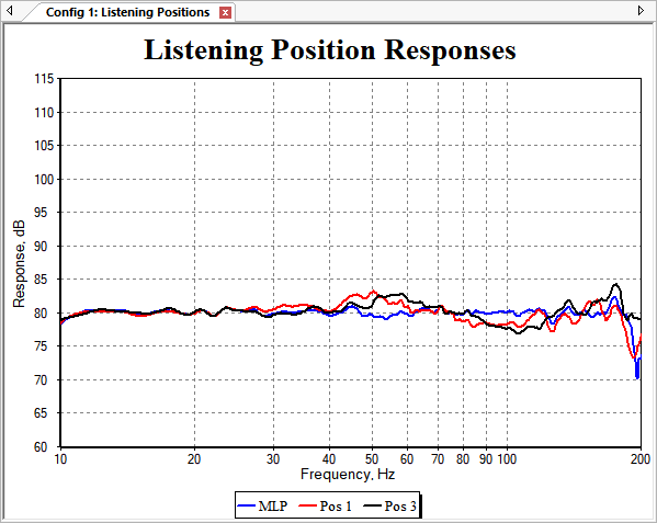
The errors for this optimization run, found using the Performance Metrics dialog, are shown below.

Errors after multi-stage optimization:
SPL penalty: 2.76 dB
STSV: 0.70 dB
MLP target error: 0.52 dB

Comparing to Previous Results

Let's compare these results with the previous two optimization runs by looking at the graphs and numerical data.

Optimizing Just the SPL and MLP Flatness

When we optimized for maximum SPL, then for MLP flatness without taking STSV into account, we got the following result.

The errors from the Performance Metrics dialog are shown below.

Errors after optimization with maximized SPL and flattened MLP:
SPL penalty: 1.84 dB
STSV: 1.98 dB
MLP target error: 1.01 dB

For this example, the multi-stage optimization approach takes a modest hit of less than 1 dB on the SPL penalty, but gets solid improvements in STSV and MLP target error compared to the method that takes only SPL penalty and MLP flatness error into account. This is easily seen from both the graphs and the numerical data.

Optimizing Just the STSV and MLP Flatness

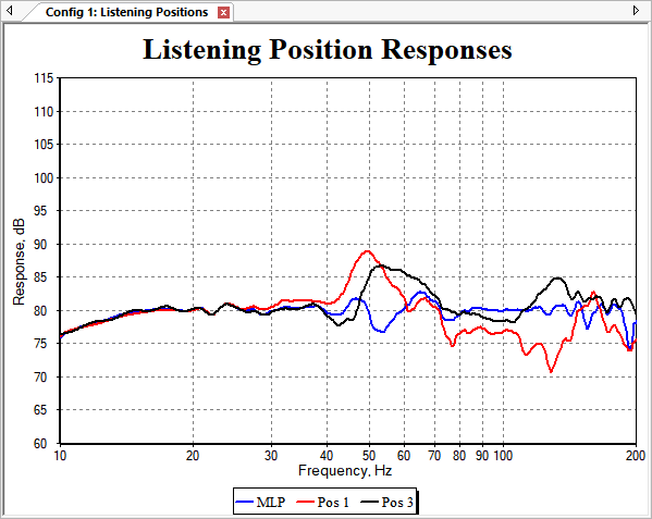
When we ran a traditional MSO optimization, which takes only STSV and MLP flatness into account, we got the following result.

This graph is impressive looking, showing vary low MLP flatness and STSV errors. But the numerical data shown below reveals that we took a substantial hit on the SPL penalty in order to achieve those goals.

Errors after traditional optimization for STSV and MLP Flatness:
SPL penalty: 7.15 dB
STSV: 0.31 dB
MLP target error: 0.27 dB

The results above for the composite optimization approach show that we've obtained useful improvements in STSV and MLP target error in exchange for a modest concession in SPL penalty. The various compromises between low MLP flatness and STSV errors on the one hand, and low SPL penalty on the other are ultimately the user's choice. However, many users, especially those of expensive high-performance subwoofer systems, aren't willing to sacrifice much SPL capability for consistent performance from seat to seat. Experimenting with different compromises via the multi-stage optimization approach of MSO is a useful way to deal with that dilemma.

Some Additional Possibilities

Later in the User Guide, the use of multiple configurations as well as optimizing multiple configurations in a single step will be discussed. One possibility to further explore the trade-offs between STSV errors and SPL penalty is to create several different configurations that differ by only one thing: the Allow sub PEQs to increase SPL penalty by not more than option value on the Multi-Stage Options property page of the Optimization Options property sheet. This is illustrated below.

By creating a family of configurations that have a range of values for this parameter, you can use MSO's multiple-configuration optimization feature to get a family of compromises between STSV and SPL penalty, allowing you to find one or more solutions that meet your needs.

But before discussing such features as multiple configurations, we need to first establish the requirements for the measurement data we supply to MSO, so we can ensure that MSO's performance predictions are as close as possible to what we actually measure when we verify the performance of the system. That's the subject of the next topic.