Optimization of Multiple Configurations
Optimizing Multiple Configurations in a Single Run
In prior examples, we've been optimizing configurations one at a time by right-clicking the configuration in the Config View and choosing Optimize Configuration. Then we explored having multiple configurations, but only for the purpose of graphical comparison of the results of configurations that had already been optimized one at a time. In this example, we'll show how to set up multiple configurations with different compromises allowed between SPL penalty and seat-to-seat variation, then use the Multiple-Configuration Optimization Dialog to perform, in a single run, multiple optimizations of all the configurations we set up in this way.
The Steps to be Performed
Downloading the User Guide Examples: The data for this demonstration are available as getting_started_user_guide.zip. To get results that match the examples, please download and unzip this file before beginning if you haven't already.
Open up the user-guide-5.msop project from the earlier multi-stage optimization example and save it as user-guide-8.msop to avoid accidental overwriting of the original project later. We're going to perform the following steps with this new project.
- Rename the Config 1 configuration to Alternative 1.
- Set the optimization options of Alternative 1 specify that a multi-stage optimization is to be run on it, and specify other options to be appropriate for that optimization type.
- Run some test optimizations of Alternative 1 to make sure they're working as planned. Make appropriate changes as necessary.
- After a successful test optimization, clone Alternative 1 multiple times to create a family of configurations to be optimized.
- For each configuration cloned as above, set a different allowable compromise between SPL penalty and seat-to-seat variation on the Multi-Stage Options property page of the Optimization Options property sheet.
- Launch the Multiple-Configuration Optimization Dialog and specify that the cloned configurations created above are to be optimized.
- Run the multiple-configuration optimization.
- Compare the results in the Configuration Performance Metrics dialog.
Renaming the Config 1 Configuration
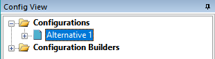
In the Config View, select the Config 1 configuration, press F2 and edit its name to be Alternative 1.
Let's have a look at the Data View to see what changes were made to the graphs.
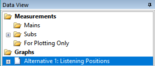
The graph named Config 1: Listening Positions has been automatically renamed to Alternative 1: Listening Positions.
Setting the Optimization Options of the Prototype Configuration
Rather than cloning our Alternative 1 configuration right away, we'll set its optimization options first instead. That way, we can make any desired changes to its optimization options, so that when we finally do clone Alternative 1, the good optimization options will be cloned as well. If we were to immediately clone Alternative 1 without first getting its optimization options right, we'd need to fix the optimization options of all of the clones one at a time. That would be a lot of unnecessary work.
For setting up the optimization options of this example, we'll rely heavily on the previous example of multi-stage optimization. More detail is provided in that example, so if you need further explanations about any specific options, check out that topic. We'll use all the same options as that example, so the illustrations from that section will be reused here. Some of these illustrations show the configuration name to be Config 1 from the prior example, so you'll just need to mentally replace that name with Alternative 1 for this example.
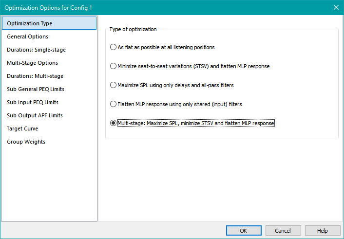
First, open up the Optimization Options property sheet for the Alternative 1 configuration. The Optimization Type property page will be shown. Set it as below.
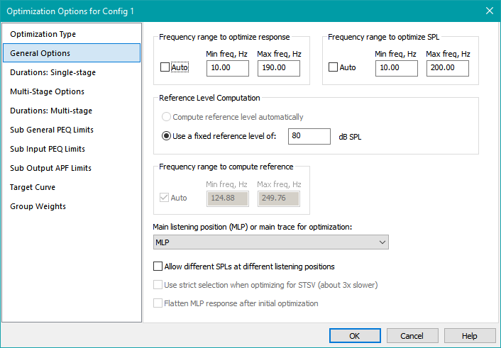
The General Options need to be set next. Open up the General Options property page and set it as below.
Next, set the options on the Multi-Stage Options property page. For the fastest possible optimization, uncheck the Use strict selection when optimizing for STSV option on this page. The options should be as shown below.
The optimization durations are set next. Set them as below.
Next, the parameter limits for the output PEQs are set on the Sub General PEQ Limits property page. Set these limits as shown below.
The input PEQ parameter limits are set using the Sub Input PEQ Limits property page. These limits should be set as shown below.
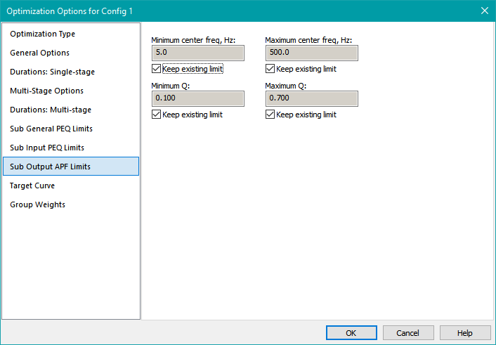
Finally, the output all-pass filter parameter limits should be set using the Sub Output APF Limits property page. Set them as below.
Click OK to accept all the information you've entered.
Running a Trial Optimization
Now we can try a test optimization. On the Multi-Stage Options property page, we previously disabled the Use strict selection when optimizing for STSV option. This trial optimization will test to see if that change was reasonable to make.
In the Config View, right-click on the Alternative 1 configuration and choose Optimize Configuration. The following result was obtained.
This result compares favorably with the one from the earlier multi-stage optimization example, so we can conclude that disabling the Use strict selection when optimizing for STSV option as we did above was a good choice.
Cloning the Prototype Configuration
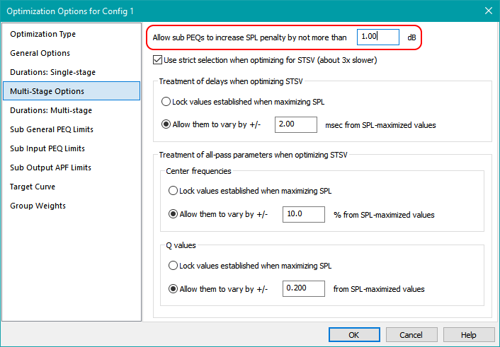
Our goal for this example is to explore various compromises between SPL penalty and seat-to-seat variation (STSV) using the multiple configuration optimization feature. We'll do this by first cloning the Alternative 1 configuration multiple times until we end up with configurations named Alternative 1, Alternative 2, Alternative 3, Alternative 4, Alternative 5 and Alternative 6. For each of these alternatives, we'll enter a different value for the Allow sub PEQs to increase SPL penalty by not more than option on the Multi-Stage Options property page of the Optimization Options property sheet. This option is illustrated below.
Then we'll run a multiple-configuration optimization, which will optimize all six configurations. Afterward, we'll examine how the compromises between SPL penalty and STSV work out.
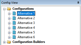
First, we need to clone the Alternative 1 configuration. Right-click on it and choose Clone Configuration. In the Clone Configuration dialog box (not shown), enter Alternative 2 for the new configuration name and make sure the Clone associated graphs checkbox is checked. Repeat this process until you end up with configurations named Alternative 1, Alternative 2, Alternative 3, Alternative 4, Alternative 5 and Alternative 6. The Config View should look as below.
Let's see how the Data View turned out. It's shown below.
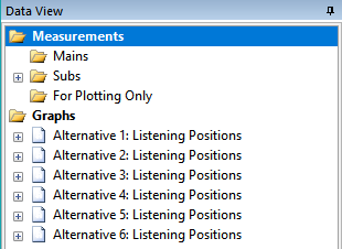
In cloning the configurations, MSO has automatically named the new graphs to match the new configuration names, so there's no need to change the graph names.
Now we'll need to make a change to the optimization options for the six configurations. For each one, a different value will be entered for the Allow sub PEQs to increase SPL penalty by not more than option on the Multi-Stage Options property page of the Optimization Options property sheet shown above. Use the values summarized in the table below.
| Configuration Name | Allowed SPL Penalty Increase |
|---|---|
| Alternative 1 | 0.25 dB |
| Alternative 2 | 0.50 dB |
| Alternative 3 | 0.75 dB |
| Alternative 4 | 1.00 dB |
| Alternative 5 | 1.25 dB |
| Alternative 6 | 1.50 dB |
Allowed SPL Penalty Increase for Each Configuration
This requires opening up the Optimization Options property sheet for each configuration. When you're done, double-check the value of this option for each configuration against the value in the table above. Before running the optimization, save the project as user-guide-8.msop.
Running an Optimization on All Configurations
Next, we'll optimize all the configurations at once. To do that, choose Config, Optimize Multiple from the main menu. The dialog shown below will be launched.
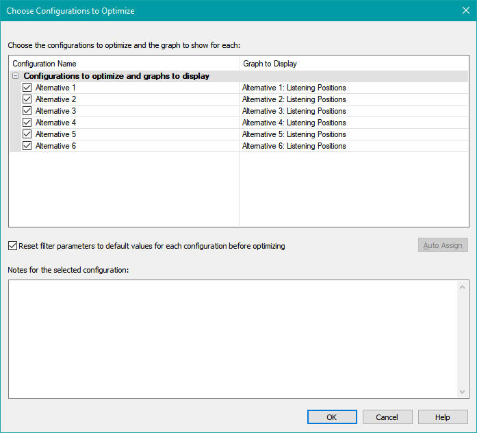
Use the checkboxes to select all the configurations as above. In the right column, there is a choice for which graph you wish to show when optimizing the configuration. If there is more than one graph containing traces that refer to the configuration on its left, the combo box will allow you to choose which one you want to show. Since there is only one graph for each configuration, the default is correct.
When you press OK, the optimization will start. This run will take a long time, as multi-stage optimization is the most complex type supported by MSO, and there are six configurations to optimize.
A Summary of Optimized Results
A summary of results from the downloadable examples is shown in the table below.
| Configuration Name | SPL Penalty | STSV |
|---|---|---|
| Alternative 1 | 2.08 dB | 0.98 dB |
| Alternative 2 | 2.34 dB | 0.94 dB |
| Alternative 3 | 2.50 dB | 0.81 dB |
| Alternative 4 | 2.84 dB | 0.73 dB |
| Alternative 5 | 3.01 dB | 0.65 dB |
| Alternative 6 | 3.34 dB | 0.63 dB |
STSV vs. SPL Penalty for Six Configurations
The data are shown in plot form below.
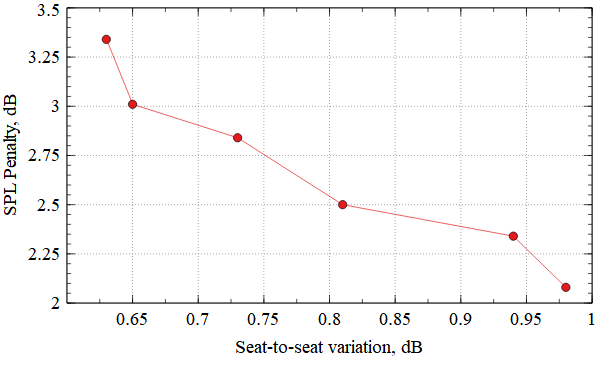
Alternative 4 is a reasonable choice. Its SPL penalty of 2.84 dB is 1 dB worse than the best that can be achieved with equal gains for all subs at all frequencies with all-pass filters to fix up the relative phase of the subs. It can be seen from the left side of the graph that attempts to further decrease the STSV result in the SPL penalty rising quickly.
Comparing the Results to the Condition Before Optimization
In an earlier part of the user guide, we looked at the errors of this same configuration prior to any optimization. The conditions before optimization were flat gains in all sub channels at all frequencies, zero delays and identical all-pass filters in all channels (giving matched phase of the DSP filter channels at all frequencies). The error data were displayed in the Configuration Performance Metrics dialog as shown below.
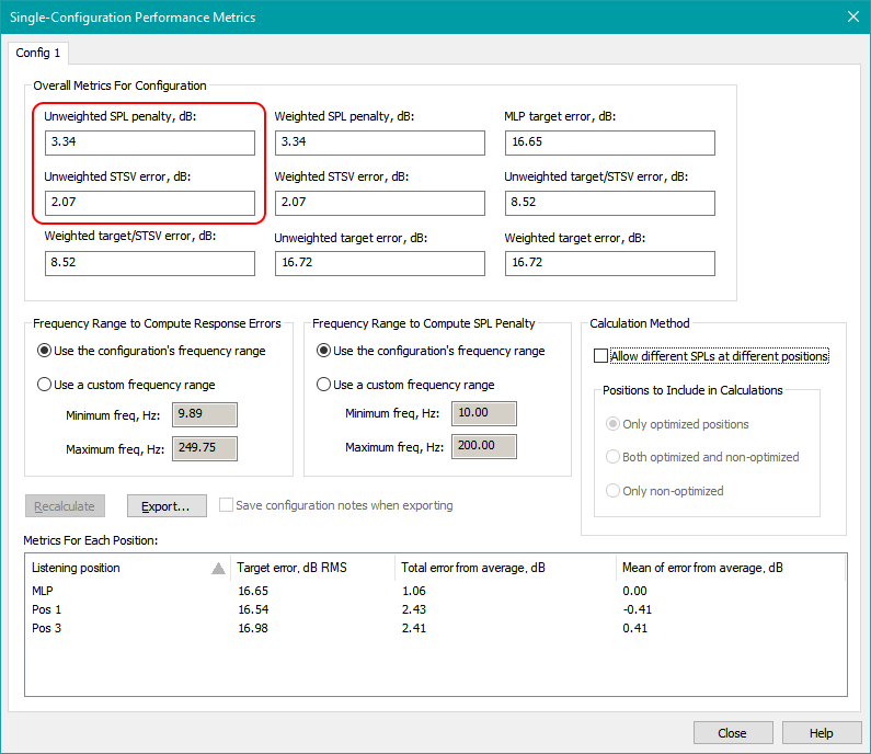
One interesting aspect of this data is that the SPL penalty value of 3.34 dB is the same as that of Alternative 6 in the table above - the configuration with the worst SPL penalty of the group.
We'll look at more specific information about the Configuration Performance Metrics dialog in the next topic.