Introduction to Multiple Configurations
Comparing Results From Different Optimizations
So far, when showing results from different optimizations, we've just used separate project files. That method isn't very effective, but using it for the early examples allowed us to concentrate on the different types of optimization available before introducing the complexity of multiple configurations. Since we've covered all the important optimization types, now is a good time to introduce multiple-configuration techniques for comparing different results.
Comparing Before and After Using the High-Frequency Roll-Off Example
Downloading the User Guide Examples: The data for this demonstration are available as getting_started_user_guide.zip. To get results that match the examples, please download and unzip this file before beginning if you haven't already.
The previous example of flattening out the high-frequency roll-off of the MLP produces its results in a simple form, making it an easy first example to compare the results of optimizing multiple configurations.
Open up the user-guide-6.msop project and save it as user-guide-7.msop to avoid accidentally overwriting the original project.
Cloning the Existing Configuration
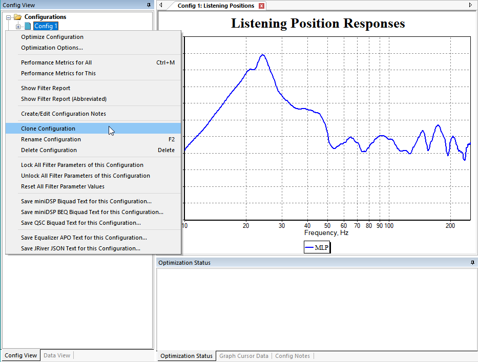
In the Config View, right-click the Config 1 configuration and choose Clone Configuration as shown below.
The Clone Configuration dialog will be shown as below.
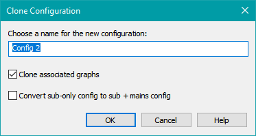
The new configuration will be called Config 2. The Clone associated graphs option causes all graphs having data traces referring to Config 1 to be replicated, but with all references to Config 1 data in the original graph changed to refer to Config 2 (the new configuration name) in the new graphs. Accept the defaults and press OK.
We now have two identical configurations, but we want to compare the results obtained before and after flattening the high-frequency response. The only difference between the before and after conditions was the addition of the HF Shelf Linkwitz Transform filter and the optimization of its parameter values. If we were to delete this filter from Config 1, that would take Config 1 back to the baseline condition from before optimization. Let's delete that filter now.
Expand the Config 1 node in the Config View and locate the HF Shelf Linkwitz Transform filter FL53. We locked that filter after the optimization. The locking operation turns the filter's icon dark gray, so it should be easy to find. Right-click on this filter and choose Delete Filter as below, or just select it and press the Delete key.
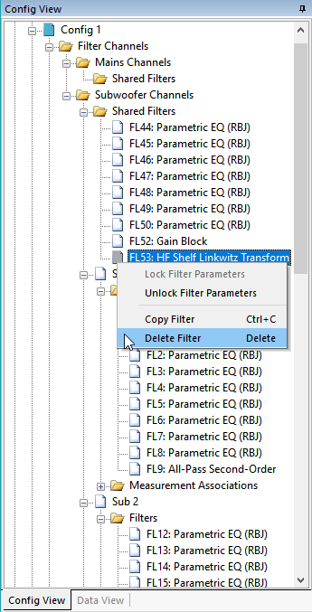
Removing the HF shelving filter from Config 1 means that it now reflects the baseline condition from before our previous optimization, while Config 2 gives us the results after. We should really rename these configurations so the new names reflect the conditions they show.
Renaming Items in the Config View and the Data View
Before we rename the Config 1 and Config 2 configurations, let's first have a look at what happened to the Data View after cloning Config 1. It should be as shown in the image below.
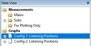
Before we cloned Config 1, there was only one graph. Now there are two because we chose the Clone associated graphs option on the Clone Configuration dialog. The name of the newly created graph for Config 2 was automatically chosen by MSO to be similar to that of the graph for Config 1.
Renaming items in MSO's tree views is done the same way you rename files and folders in the Windows File Explorer. Just select the item, press F2 (or click twice without double-clicking), and then you can edit the item's name in place. Using this technique, rename "Config 1" to "Baseline" and "Config 2" to "Flattened" as shown below.

Now let's go into the Data View to see if we have to make any changes to the graph items. The graph items in the Data View should look as below.
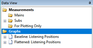
Renaming the configurations has caused their associated graphs to be automatically renamed by MSO as well.
Now we have two graphs, with each one showing data from a different configuration. If either of the graphs aren't shown, select the name of the one you want to show, right-click and choose Show Graph.
Having separate graphs in this way is still not convenient though. We'd like to have a single graph that shows the relevant traces from both configurations. We could right-click on the Graphs node above and choose New Graph, but if we did that we'd have to set all the options for axis limits, dB per division and so on. The graphs we have are already set up with these options the way we want them.
Cloning the Baseline: Listening Positions Graph
Instead of creating a new graph from scratch, let's clone the Baseline: Listening Positions graph. Right-click on this graph's name and choose Clone Graph as shown below.
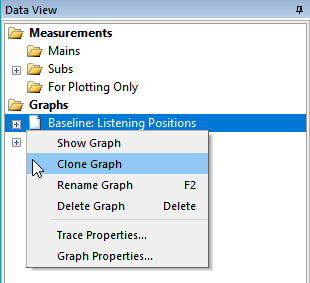
This will create and show a new graph called "Copy of Baseline: Listening Positions". In the Data View, expand the node of this graph so that all the graph traces are shown as below.
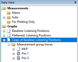
We want to end up with two traces on the graph: the MLP from the configuration called Baseline and the MLP from the configuration named Flattened. All traces on a graph must have unique names, so we can't have two traces called MLP. This suggests renaming each MLP trace with information that specifies what configuration it's from. Also, the new graph name was automatically created. We'd like to choose a more descriptive name. Finally, there's two traces (Pos 1 and Pos 3) whose visibility is toggled off. We can just delete those. Perform the following steps.
- Select each of the trace names Pos 1 and Pos 3 and press the Delete key to delete them.
- Select the trace named MLP, and using the same renaming techniques we've been using, rename it to MLP Baseline.
- Select the name of the graph called Copy of Baseline: Listening Positions and rename it to MLP Baseline vs. Flattened.
The data view should now look as below.
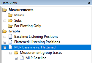
Adding a New Trace and Renaming it in a Different Way
Now the graph and the baseline MLP trace are named as we want them to be, but we still need to add the MLP trace from the Flattened configuration. To do that, we need to launch the Graph Properties property sheet for the newly renamed MLP Baseline vs. Flattened graph. If this graph is not the active one, right-click on MLP Baseline vs. Flattened and choose Show Graph. Then press Ctrl+G to launch the Graph Properties property sheet.
Select Measurement Groups under Trace Data Types. Check the trace for the configuration named Flattened and measurement group named MLP as shown.
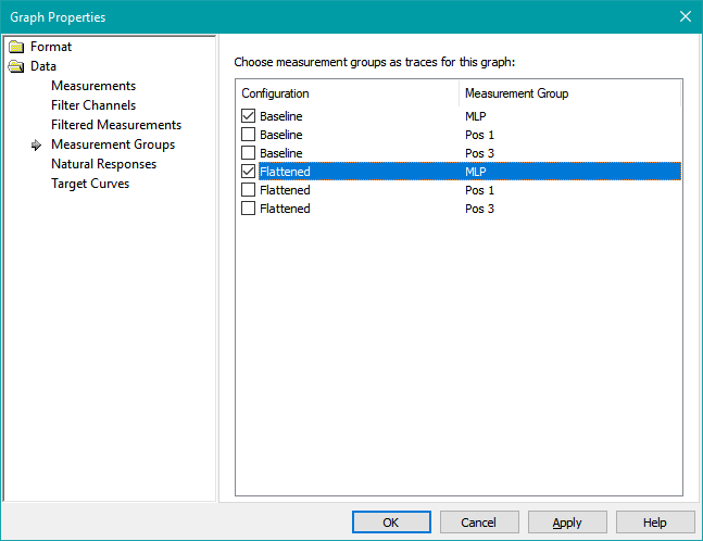
Press Apply to accept the change. A new trace tree node will appear under Trace Properties. If it can't be seen, click on Trace Properties to expand it. The trace added by this process has been automatically named to Pos: Flattened: MLP as shown below.
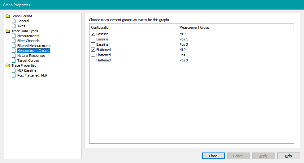
We'd like to have a better name for this new trace. Since the original trace was called MLP Baseline, let's call the new one MLP Flattened. To change its name, select it in the tree view on the left as shown and press F2 to edit it. After entering the new name, the result will look as below.
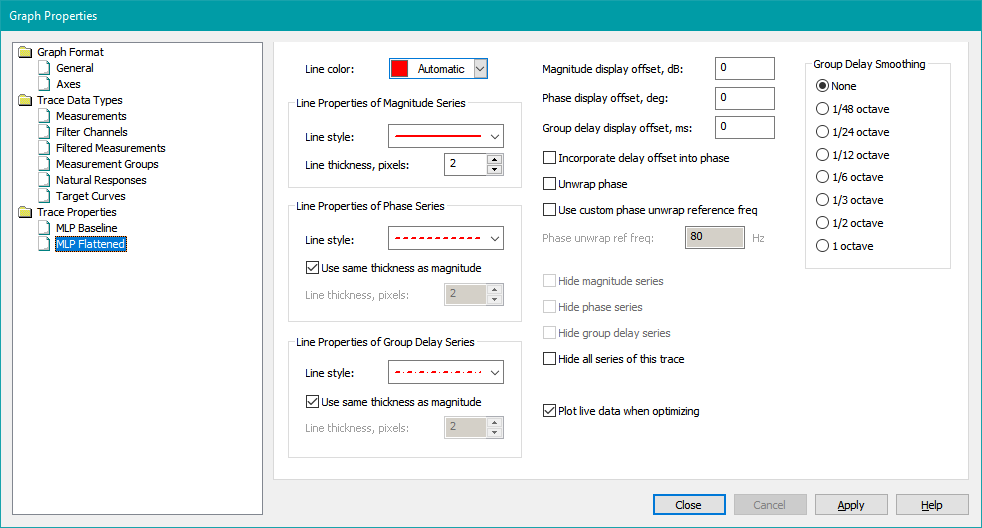
Notice that when selecting the trace node under Trace Properties on the left, the property page for that trace is made active on the right, allowing you to specify properties such as line color, thickness, and style for the selected trace. We'll just keep the defaults for now. Press Close to accept and finalize all the changes.
The changes we just made will also be reflected in the Data View as shown below.
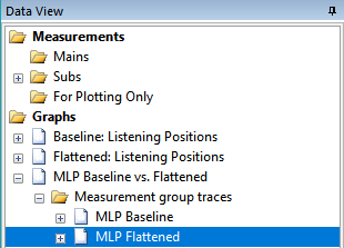
After having done all this, let's see how the graph looks. Use the command discussed earlier to show the graph if it isn't visible. It should look like the image below.
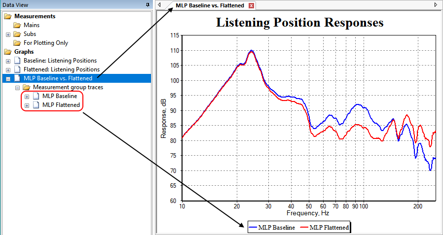
By comparing the graph and the Data View, we can see the relationship between the components of the graph as shown in the Data View with the graph itself. In the Data View, the name that we picked for the graph (MLP Baseline vs. Flattened), appears in the graph window's tab. The names that we picked for the traces, MLP Baseline and MLP Flattened, appear in the legend. Now that we have the before and after conditions shown on the graph, we can see the effect that a single HF Shelf Linkwitz Transform filter can have on the response. The HF Shelf Linkwitz Transform filter packs a lot of equalization power into a single filter.
Since the modifications to this project are complete, save it as user-guide-7.msop.