Getting Started With Graphs
Picking up Where We Left Off
In the previous sections, we walked through the Measurement Import Wizard and the Configuration Wizard to create a project with a single configuration. We saved the project as getting-started-1.msop. We'll customize the wizard-created graph of that project to improve its appearance and usefulness.
If you didn't save this project earlier, you can find a copy by downloading and unzipping the Getting Started files. Before continuing, save this project as getting-started-2.msop. This will preserve the project for later use.
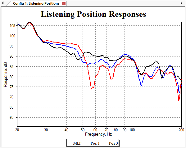
Each project (.msop file) also has a .msow file associated with it. The .msow file contains information about what kind of tabbed windows were displayed when the project was saved (or even closed without saving). If the .msow file is not present in the same directory as the .msop file, no tabbed windows will be displayed. Should this occur, go to the main menu, choose Graph, Show Graphs, check the graphs you want shown and choose OK. This will show the graph, pictured below, that we created earlier.
Modifying the Appearance of Graphs
Right-clicking on the graph shows its context menu.
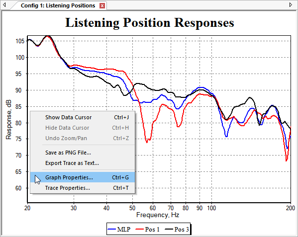
Invoking the Graph Properties command allows you to customize both the graph itself (axes, legend etc.), and each trace of the graph (color, line thickness, offset and so on). Rather than using the context menu, it's quicker to just use the Ctrl+G shortcut key.
Choosing Graph Properties brings up its property sheet illustrated below.
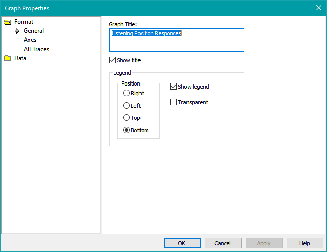
All options on this property page (show the title and show the legend on the bottom) look reasonable, so we'll keep them as-is.
Next, we'll assign the graph axes to the plot series types we want to display. We'll also specify some properties of the axes themselves, such as whether to automatically scale them, what their limits should be if they're manually scaled, and their vertical units per division. Both of these tasks are done using the Axes property page shown below.
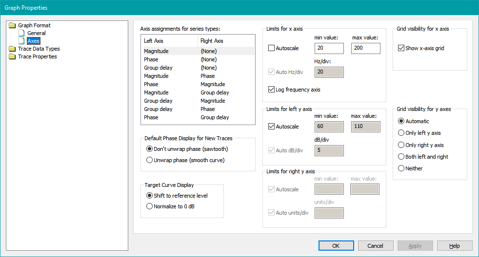
To move the keyboard focus from the tree view on the left to the property page on the right, just press the Tab key.
Here we see the default is automatically chosen, which puts the trace magnitude in dB on the left y axis, and nothing on the right y axis. We'll keep the default.
Other options are also available:
- Default Phase Display for New Traces specifies what newly-created phase traces will look like. This can be either the typical display that has a sawtooth shape and is limited to 0±180°, or a continuous curve that spans a wide range of angles. This setting does not affect the format of existing phase traces. To change that on a per-trace basis, you can use the Trace Properties property page for the desired trace, which we'll look at shortly.
- Target curves that you specify (elsewhere in MSO) can be displayed on MSO graphs. The Target Curve Display option relates to how these curves appear on graphs. For instance, if your target curve text file shows +6 dB at 20 Hz and 0 dB at 200 Hz, Normalize to 0 dB will show the curve as-is. The Optimization Options property sheet (not yet discussed) in most cases requires you to specify a reference level, which is the SPL value that MSO tries to force your response to match during optimization. When Shift to reference level is specified, and a reference level of, say, 80 dB is specified, the target curve just described would show 80 dB at 200 Hz and 86 dB at 20 Hz. This has the advantage of allowing you to see the MLP response being forced to the target curve as an optimization is run. Please note that the reference level in MSO has nothing whatsoever to do with AVR reference levels.
We won't be doing any optimization in the Getting Started Guide, as this guide is mainly for familiarizing you with MSO. We'll keep these options at their defaults.
Next, we'll look at the axis parameters themselves. These are specified on the right side of the Axes property page above.
Looking at the graph at the top of this page, we can see a few things that should be changed.
- For online forum posting, a de facto standard is to show magnitude response graphs with their vertical axis set to 5 dB per division (dB/div). Although the image does show 5 dB/div, this value isn't guaranteed. It's determined by y-axis auto-scaling and varies with the size of the window and the monitor's pixel resolution. We should manually force this to the common 5 dB/div value.
- The minimum and maximum values of the graph's y axis are strange values determined by the y-axis auto-scaling. They should each be set to a multiple of the chosen dB/div for a clean appearance. Since we'll be using 5 dB/div, we'll set both y-axis limits to multiples of 5.
- Some low-frequency data is being cut off. Our data goes down a bit lower than 10 Hz, but the MSO default limits for the frequency axis are 20 Hz to 200 Hz. We'll change the lower frequency limit to 10 Hz.
Incorporating these changes to the Axes property page gives us the result below.
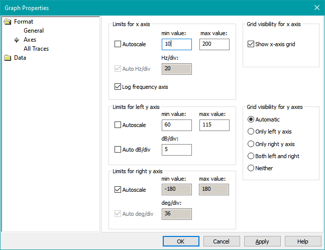
The minimum value of the frequency axis has been set to 10. For the left y axis, Autoscale has been unchecked, allowing the minimum and maximum y-axis values to be set to 60 and 115 dB respectively. Unchecking y-axis Autoscale has allowed Auto dB/div to be unchecked, which permits the left y-axis dB/div to be forced to 5.
All the options for Limits for right y axis are disabled, since no data is associated with the right y axis.
We don't need to press OK to see the changes. Instead, we can choose Apply, which will apply the changes while keeping the dialog up. If we don't like the appearance or if we forget something, we can make more changes while checking the result with Apply until we get the appearance we want.
Here's what we get with the above changes.
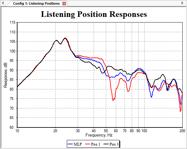
This looks a lot better than our original graph at the top of the page.
If you haven't done so already, choose OK to close the Graph Properties property sheet. Before continuing, save this project as getting-started-2.msop. You can also get a copy of the project with the modifications we did above in the Getting Started files you downloaded earlier. Look for the getting-started-2.msop project in the zip file.
Modifying the Appearance of Graph Traces and Series
In addition to the options for controlling the appearance of the graph itself, you can control the appearance of graph traces and the individual series of each trace. This is also done using the Graph Properties property sheet. Launch it as before, using the graph's context menu or the Ctrl+G keyboard shortcut.
To activate the Trace Properties property page, you can either scroll down the tree view on the left using the keyboard, or use the mouse to select the tree's Trace Properties node. This will cause the Trace Properties node to expand to show a node for each trace. Selecting the desired trace allows you to change its properties.
In the Trace Properties property page shown below, a trace refers collectively to all the data that can be plotted for the chosen quantity (in this example, the response at the MLP), while a series refers individually to each plot line that can be derived from the data (such as Magnitude, Phase, and Group Delay).
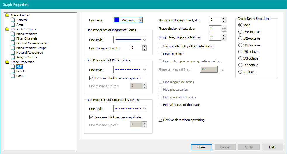
In the image above, Line Color is a property of the trace, since all series of a trace (Magnitude, Phase, and Group Delay) have the same color. On the other hand, Line Style is a property of each series, since this is specified individually for each of the Magnitude, Phase, and Group Delay series.
Changes Made on the Trace Properties Property Page Are Immediate
For other property pages of the Graph Properties property sheet, you must first make all the changes you want to the controls on the page. This enables the Apply button. Then you must either press Apply for these changes to take effect, or navigate to another property page (which performs the same action as pressing Apply).
The Trace Properties property page is different. As you make changes to controls on this property page, they are detected and applied immediately. This makes customizing graph traces and series faster.
Some Sample Changes to Series Appearance
There are many options here, but for now we'll only look at trace thickness and color, along with offsets for the individual trace series.
Activating the Trace color combo box brings up a Windows color picker for your color choice. You can also tell the color picker to use the default, which is an automatically generated color.
You can set the Line thickness, pixels to the desired value via the spin button control. As you change the thickness, the Line style combo box display changes to show a line with the actual thickness and chosen line style exactly as it will appear on the graph. The default line thickness is two pixels, which may be too thin if your computer has a 4k display.
You can apply offsets to the magnitude, phase, and group delay series of the trace. We'll just look at the magnitude for now, since that's the only date being displayed.
Magnitude display offset, dB is usually used when plotting data from multiple configurations on a single graph. That will be discussed later in the User Guide. Briefly, by offsetting all the curves from one configuration by the same value relative to the other, visual comparison of data from multiple configurations is made easier.
As a quick demonstration, we'll change the magnitude offset and trace thickness of the MLP trace. Select the MLP trace on the left, and enter -10 for the value of Magnitude display offset, dB. Set Trace thickness, pixels to a value of 4.
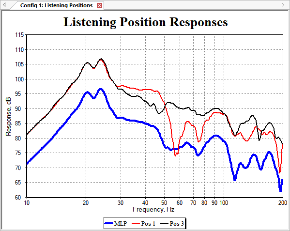
This change doesn't have any practical usage in this specific situation, so there's no reason to save the project in this state.
What's Next
The purpose of the Getting Started Guide has been to familiarize you with the simplest basics of how to begin using MSO. We haven't covered optimization yet. Understanding MSO's optimization capabilities and what you can do with them requires some in-depth technical explanations. Such matters are the subject of the User Guide.