How Optimization Errors are Calculated: the Details

Error Calculation Details

This topic builds on earlier discussion of MSO's error calculations given in the description of the Configuration Metrics Dialog. It's a good idea to become familiar with that dialog if you haven't done so already. This topic attempts to describe not only what calculations are performed, but in some cases also why.

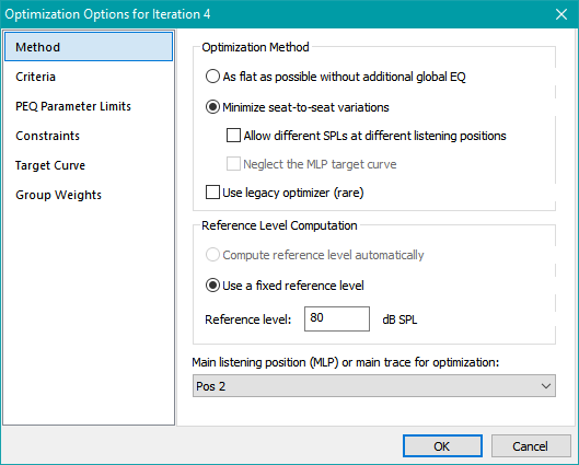
MSO is used with DSP hardware containing simple IIR filters such as PEQ and shelving filters. The PEQ filters are used to counteract room modes, while the other filter types are used for overall response shaping, such as for matching a response to a target curve. MSO works by adjusting filter parameter values, as well as gains and delays, to minimize a calculated error. There are different methods of calculating this error, depending on the optimization method selected in the Optimization Type property page of the Optimization Options dialog shown below. See also the documentation for this property page for other details about it.

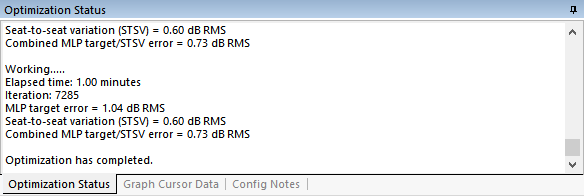
The optimization errors described in this topic are also displayed in the Optimization Status tab of the Output window when the optimization is running and after it has stopped. See the figure below for an example.

You can also display the calculated errors for any configuration in a project at any time by launching the Multiple-Configuration Performance Metrics dialog.

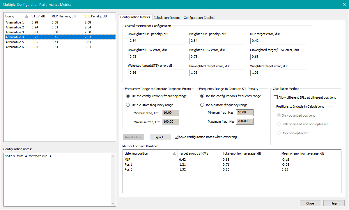
This dialog is most easily launched by pressing Ctrl+M.

Background

Up until version 1.0.46, MSO was entirely a target curve-based system. This was done to differentiate it from Harman Sound Field Management (SFM) as much as possible. That's not because of any problem with SFM, but because of its patented status. Harman SFM uses a combinatorial optimizer (that is, one using only discrete parameter values) to minimize a metric called the mean spatial variance (MSV) without regard to the frequency response of the combined sub outputs. The MSV is one possible measure of the subs' seat-to-seat response variation. After doing that, it applies global EQ to achieve the desired target curve in a separate step. In contrast, MSO uses an optimizer that allows continuous parameter adjustment within specified limits to simultaneously achieve the desired target curve and minimize seat-to-seat response variation (which is calculated using a different metric than the MSV).

What's common to MSO and SFM is the ability to have different EQ, delay, and gain/attenuation for each sub. This allows the change in frequency response after EQ is applied to vary with listening position. This property, when harnessed correctly, allows the seat-to-seat variation of the combined subs' frequency responses to be reduced. Since these seat-to-seat response variations in the modal region are caused by room modes, the ability to reverse this effect to a substantial extent has been called mode manipulation by Floyd Toole in Chapter 8 of the third edition of his book Sound Reproduction.

Details Common to All Optimization Modes

MSO works according to the Superposition Principle from Linear System Theory. The Superposition Principle relies on the idea of a complex summation. The term "complex summation" stems from the fact that complex numbers are used in its implementation.

Complex Summations Are Represented by Measurement Groups

We can think of real numbers in terms of a number line, and the "angle" of a real number as being measured, like in trigonometry, relative to the positive portion of the number line. The number zero is assumed to be at the origin of this one-dimensional coordinate system. In this interpretation, real numbers can have only two possible angle values: 0 degrees for positive numbers and 180 degrees for negative ones. The magnitude of a real number r, which can be interpreted geometrically as its length, is its absolute value and is written as |r|.

We use complex numbers to represent numbers that have a magnitude (length) and angle, where the angle can now take on any value in the range 0±180 degrees, not just 0 or 180 degrees as in the case of real numbers. This means we can view them as being in a plane, like the x-y plane considered in trigonometry. This plane is called the complex plane. A complex number z is written (by engineers and physicists) as z = u+jv, where u (a real number) is called the real part of the complex number, v (also a real number) is called the imaginary part of the complex number, and j=sqrt(-1). Here, j, called an imaginary number, which is a complex number whose real part is zero. Mathematicians use the letter i for sqrt(-1). The x-axis of the complex plane is called its real axis, and the y-axis is called its imaginary axis. The imaginary axis is sometimes called the j-axis. The magnitude of a complex number z is its length, and is usually written as |z| by analogy with the absolute value (length) of a real number. When a complex number z is written as z = u+jv, its magnitude (that is, length) |z| can be computed as:

|z| = sqrt(u² + v²),

which is just the Pythagorean Theorem for computing the length of the hypotenuse of a right triangle. For the number j=sqrt(-1) by itself, we have u = 0 and v = 1. So then we have:

|j| = sqrt(0² + 1²) = 1

The angle of the complex number z, which for some reason is called arg(z), and to which we'll assign the symbol θ, is given by

θ = arg(z) = atan2(v, u)

where atan2() is a four-quadrant arctangent function.

To find the angle of the number j=sqrt(-1), we can use the above formula as follows:

θ = arg(j) = atan2(1, 0) = π/2 radians = 90 degrees

This reinforces the idea that the j-axis is the vertical axis of the complex plane.

The real part u and the imaginary part v of z are sometimes written as Re(z) and Im(z) respectively as follows.
u = Re(z)
and
v = Im(z)

Finally, the real and imaginary parts of z can be written in terms of its magnitude |z| and angle θ as follows.
Re(z) = |z| * cos(θ)
Im(z) = |z| * sin(θ)

The rules for complex summation are very simple. If we have two complex numbers
z₁ = u₁+jv₁
and
z₂ = u₂+jv₂
Their sum z₁ + z₂ is given by
z₁ + z₂ = (u₁+u₂) + j(v₁+v₂)

The rules for complex addition can be summarized as, "the real part of the sum is the sum of the real parts, and the imaginary part of the sum is the sum of the imaginary parts." This idea is straightforwardly extended to the summation of any number of complex values.

In MSO, a collection of measurements we wish to add up using the complex summation rules above is represented by a Measurement Group. Prior to the complex summation of the measurements in the group, each raw measured sub or satellite response is first altered by the frequency response of the filter channel associated with it, including both magnitude and phase of each filter channel response. In the vast majority of cases, a measurement group corresponds to a listening position, but in another topic we'll talk about a special usage for which this is not the case.

Let's take a specific example in which each measurement group corresponds to a listening position, and the measurements which make up the group are all sub measurements. If you had, say, four subs and five listening positions, you'd have five measurement groups (corresponding to the five listening positions), and each measurement group would contain four measurements. Each of these four measurements in the group correspond to each of the subs measured at that position. In MSO, this means that for each pass of the optimizer (which corresponds to a collection of guesses for all the filter, delay and gain parameters), the following operations are performed:

1. The measured response of each sub is altered by the computed response of the filter channel with which that sub's measurement is associated.
2. The response format of each sub at each frequency is converted from "dB SPL and phase angle" to a complex number.
3. A complex summation of all the subs' filtered responses is performed at each frequency.
4. The complex number computed from this summation is converted back to "dB SPL and phase angle" format at each frequency.

To convert a measurement in the form of "dB SPL and phase in degrees" to a complex number, the C++ function below can be used. The notation "<double>" next to "complex" just means the complex number is of a double-precision type, while "mag" and "angRad" are double-precision real numbers representing the unitless magnitude of the complex number and its angle in radians respectively. Here you can see an application of the formulas above that express the real and imaginary parts of a complex number in terms of its magnitude and angle.

complex<double> dB_deg_to_complex(double dBval, double angDeg)
{
    const double mag = pow(10.0, dBval / 20.0);
    const double angRad = (pi / 180.0) * angDeg;
    return complex<double>(mag * cos(angRad), mag * sin(angRad));
}

To get the dB SPL and phase in degrees from a complex number so obtained, the following functions can be used.

double mag_dB(const complex<double> complexVal)
{
    return 10.0 * log10(norm(complexVal));
}

double ang_deg(const complex<double> complexVal)
{
    return (180.0 / pi) * arg(complexVal);
}

In the above code, the C++ function norm(complexVal) gives the square of the magnitude of complexVal, so the base 10 log result must be multiplied by 10.0 rather than 20.0 to convert it to dB. Also, arg(complexVal) gives the angle of complexVal in radians, so it must be converted to degrees by multiplying by 180.0/π.

After these operations are done for a given measurement group, the result for that measurement group is an array containing the combined sub responses in dB SPL at that listening position vs. frequency. Then this procedure is repeated for the next measurement group and so on until the combined frequency responses of all subs at all listening positions have been evaluated. After completing the calculations for N listening positions, there will be N arrays of SPL vs. frequency, one for each listening position. If a target curve is specified, these arrays are modified by the target curve as specified in the next section.

The above example is for a "sub-only" configuration. For a "subs+mains" configuration, the measured response of one or more satellites is added to each measurement group. When such a complex summation is performed and converted into the form of dB SPL vs. frequency, the result takes into account not only how the subs interact with one another, but also how they interact with the satellites. This technique of computing and adjusting the interactions of subs and satellites through optimization can be thought of as a generalized version of the "sub distance tweak" often discussed in home theater forums.

Details Common to Optimization Modes Supporting a Target Curve

Optimization modes that support a target curve also make use of the notion of a reference level. When the user does not specify a target curve, a flat one is used.

The reference level idea is best understood in connection with a flat target curve. Suppose a reference level of 88 dB SPL were chosen. In this case, MSO tries to force the response at each listening position to have an average value of 88 dB SPL over frequency, with as little variation over frequency from that level as possible.

But what does the reference level mean when the target curve is not flat? In this case, MSO first determines the maximum frequency f_max to be used by the optimizer (explained below).

Then, the user-provided target curve is offset so that its value at f_max is 0 dB. This modified curve is called the normalized target curve. Another step is added to the summation algorithm above. In this additional step, the normalized curve is subtracted from the computed response curve at each listening position. The optimizer then tries to force this difference to be a constant equal to the reference level value over the optimization frequency range. This achieves the desired target curve. This is illustrated by the example shown below.

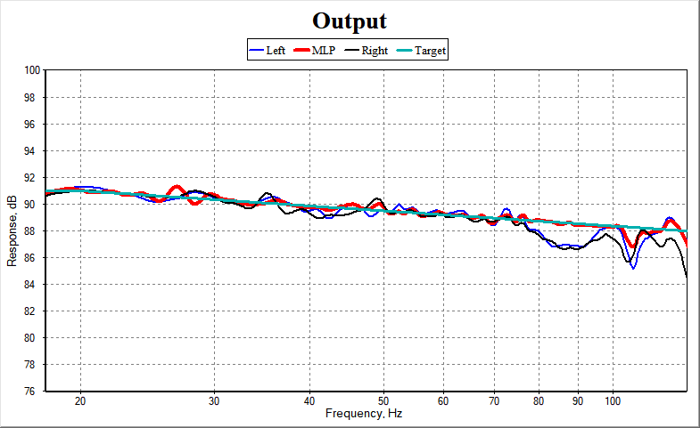
In this example, the maximum optimization frequency is 125 Hz, which is also the maximum frequency of the graph. The turquoise curve is an offset version of the target curve provided by the user, and a fixed reference value of 88 dB SPL was chosen for the optimization. It's easily seen that the SPL of the MLP (red curve) has been adjusted to be as close as possible to the actual target curve. The actual target curve is the curve provided by the user, offset so that its value at f_max is the reference level in dB (in this case 88 dB).

There are two ways of specifying the reference level: Use a fixed reference level and Compute reference level automatically.

For configurations consisting only of subs, the only available option is Use a fixed reference level. This reference level is used in connection with the target curve as explained above.

For configurations consisting of subs and satellites, chosen when you wish to optimize the integration of subs and satellites, either method of specifying the reference level can be chosen. If you choose Compute reference level automatically, additional information must be specified in the General Options property page of the Optimization Options property sheet. This is shown below.

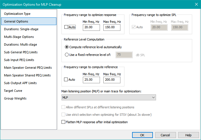
In the Frequency range to compute reference fields, you should specify the minimum and maximum frequencies to use. The reference level is then computed as follows. First, the maximum frequency used by the optimizer is computed as the larger of the maximum optimization frequency and the maximum frequency to compute the reference. In the figure above, the former value is 150 Hz and the latter is 300 Hz, so the maximum frequency used by the optimizer will be 300 Hz. Next, the target curve is normalized so its value at 300 Hz is zero dB, and in the summation algorithm above, the normalized target curve is subtracted from the computed response for each position. Here, the frequency range to compute the reference is 150 Hz to 300 Hz. The reference level is computed by taking the computed summation of all subs and specified satellites, offset by the normalized target curve, and computing its average in dB over the frequency range of 150 Hz to 300 Hz. The response in this frequency range is dominated by the satellites. The purpose of this option is to automatically compute this average level and adjust the level of the subs to match it, without the user having to guess what this level is beforehand - which would be needed when specifying a fixed reference level. Also, if additional EQ were used on the satellites to flatten their response further, this automatic calculation of the reference level takes into account shifts in the average value caused by MSO altering this EQ during an optimization. This was the original concept of MSO prior to the introduction of sub-only configurations, and MSO can still be used in this way. The technique does require care in choosing the frequency range over which to compute the reference level.

Details of As Flat as Possible at All Listening Positions Mode

When MSO was first released, this was the only optimization mode available. Many of the pieces of the computation have been described already, so they will be referenced below as needed. The data are assumed to have been taken at N_f frequencies using N_s subs and N_p listening positions. The error computation proceeds as follows.

1. First, the dB SPL vs. frequency curve at each listening position is computed according to the complex summation algorithm previously described. Recall that this procedure adds the contributions of the N_s subs at N_f frequencies for each listening position, taking phase into account.
2. Next, any non-flat target curve is subtracted from each curve of SPL vs. frequency as described above. The result at each listening position is called the offset curve for that listening position. For a perfect match of the computed SPL vs. frequency to the non-flat target curve, the offset curve would be perfectly flat.
3. For each listening position, the reference level for that position is then computed. For a fixed reference level, this level is the same for each listening position. When Compute reference level automatically is used, this reference level may differ from one listening position to the next, and from one pass of the optimizer to the next.
4. Next, for each listening position, the difference between the offset curve and the reference level is computed at each frequency. This difference at each frequency is squared, then each squared difference is accumulated into the sum of the squares of the errors over frequency for that position. This sum of squares is then divided by the number of frequencies N_f to yield the mean-squared error over frequency for each position. Then the square root of each of these mean-squared errors is taken, yielding a root-mean-square (RMS) error over frequency for each listening position.
5. At this point, we're left with N_p errors, one for each position, each of which represents the RMS error over frequency of the difference between the offset curve and the reference level for that listening position. But we need a single "magic number" representing the total error for the optimizer to do its work of error minimization.
6. To get a single number representing the total error, we take the RMS value over position of the N_p errors we've computed. That is, we square each of the N_p errors, accumulate them into the sum of squares of the errors, then divide this sum of squares by N_p to get the total mean-squared error. Finally, we take the square root of this total mean-squared error to get the total RMS error. This is the error displayed in the Optimization Status tab of the Output window as shown in the figure above.

The Distinction Between Unweighted and Weighted Flatness Errors Over Listening Position

In steps 5 and 6 above, we end up with N_p errors, one for each position, and we wish to combine them into a single error for the optimizer to minimize. Step 6 describes an unweighted RMS error computation, for which the sum of the squares of the errors is divided by N_p, the number of positions, before taking the square root. As a specific example, for N_p = 4, this calculation would look like:

error_total = sqrt(1/4(err₁² + err₂² + err₃² + err₄²))

where err₁, err₂, err₃ and err₄ are the RMS flatness errors over frequency at each listening position. This can be trivially rewritten for the unweighted case with N_p = 4 as:

error_total = sqrt((1/4)err₁² + (1/4)err₂² + (1/4)err₃² + (1/4)err₄²)

This idea can be generalized to the weighted case with N_p = 4 as follows:

error_total = sqrt(w₁*err₁² + w₂*err₂² + w₃*err₃² + w₄*err₄²)

We can see for the unweighted case that:

w₁ = w₂ = w₃ = w₄ = 1/4

and that:

w₁ + w₂ + w₃ + w₄ = 1

This property of the weights w all adding up to 1 is important. Consider a hypothetical case for which the errors at all 4 positions are equal. That is:

err₁ = err₂ = err₃ = err₄ = err

If all the weights w₁, w₂, w₃ and w₄ add up to 1, and all the errors are equal to the same value (err) we can easily see by plugging into the weighted error formula that:

error_total = err

which is exactly what we want. The weighted RMS sum of a bunch of equal errors is equal to that error. Let's take a specific example to show how MSO scales some user inputs internally before computing the weighted error. An example of unequal weighting is shown in this illustration of the Group Weights property page of the Optimization Options property sheet.

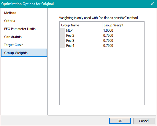
The raw values of w₁, w₂, w₃ and w₄ are 1, 3/4, 3/4 and 3/4 respectively. These don't add up to 1, though. They add up to 13/4. Before computing the weighted RMS error, MSO must normalize these values by multiplying them by 4/13. This results in:

w₁ = 4/13
w₂ = 3/13
w₃ = 3/13
w₄ = 3/13

Now the weighting factors add up to 1. In this specific case of 4 listening positions, the total weighted RMS error would be computed as:

error_total = sqrt((4/13)err₁² + (3/13)err₂² + (3/13)err₃² + (3/13)err₄²)

assuming err₁ is the RMS error over frequency of the MLP.

Of course, this technique can be easily extended to any number of listening positions. The special case of 4 listening positions was just chosen for illustration.

Addressing Seat-to-Seat Variation More Directly

Compared to using only global EQ, the As flat as possible without additional global EQ mode of MSO is a step in the right direction toward reducing seat-to-seat variation in frequency response. A hypothetical but unrealizable case is to get a perfectly flat response at all listening positions. In such a case, the seat-to-seat variation would be zero. In the real world, this is not possible. The ability to reduce seat-to-seat response variation when using the As flat as possible without additional global EQ mode is only implicit. What's needed is a way of computing the total error that explicitly includes a term that involves the seat-to-seat response variation.

Recall from the Background section that the goal of MSO is to simultaneously achieve the desired target curve and minimize seat-to-seat response variation. This suggests that the total error should consist of two components:

1. An error representing some deviation from the target curve
2. A second error representing the seat-to-seat response variation

By combining these two errors in an RMS fashion, possibly using weighting, the goal of explicitly taking into account both the response error from the target curve and the seat-to-seat response variation can be achieved. In addition, the seat-to-seat response variation error computation should avoid using the same MSV metric used by Harman SFM because of its patented status. The next section describes the specifics of the solution.

Minimize Seat-to-Seat Variations Mode

Note: the algorithm description in this section results when Minimize seat-to-seat variations mode is chosen with the Neglect the MLP target curve checkbox unchecked. The behavior when neglecting the MLP target curve (checkbox checked) is described in the next section.

The idea behind this mode is, in a sense, to reverse the emphasis from the As flat as possible without additional global EQ mode. Instead of explicitly trying to get the responses at all listening positions to match the target, thereby implicitly reducing seat-to-seat variation, the Minimize seat-to-seat variations mode explicitly tries to get a single response to match the target curve, while also explicitly trying to minimize a metric representing the seat-to-seat variation. In this way, this mode implicitly tries to get all response curves to match the target.

Calculating the Error of the MLP From the Target

Making this change requires designating a main listening position or MLP. It is only the MLP whose error from the target curve is computed. This error is computed according to steps 1 through 4 of the algorithm for calculating the error from the target curve, except that the computation of this error is only performed for the MLP. This MLP-only calculation yields a single error value, so there is no need to perform steps 5 and 6 of the above algorithm. The result of this calculation is the error in dB of the MLP response from the target curve, which will be designated error_MLP-tgt.

Calculating the Average Curve and Seat-to-Seat Variation

A measure of the seat-to-seat variation that's independent of any user-supplied target curve needs to be established. Suppose that after the responses at all listening positions were computed, the average curve were also computed. This average would be computed at each frequency as the average of the computed dB SPL values at each listening position. That is, the average is computed without regard to phase. If the computed curves at all listening positions perfectly matched the average curve, the seat-to-seat variation would be zero, even if none of the curves matched the target curve particularly well. This suggests computing the seat-to-seat variation in a way that's similar to the algorithm for calculating the error from the target curve, except that the target curve would be the average of the computed curves of dB SPL vs. frequency at each listening position. This means that the method for calculating the seat-to-seat response variation is still target curve-based, but the target curve, which is now the average of all computed curves, changes on each pass of the optimizer. With this idea in mind, we can specify the algorithm for computing the seat-to-seat variation.

1. First, the dB SPL vs. frequency curve at each listening position is computed according to the complex summation algorithm previously described. That procedure adds the contributions of the N_s subs at N_f frequencies for each listening position, taking phase into account.
2. Next, the average curve is computed. At each of N_f frequencies, the average of the dB SPL values for each of the N_p listening positions is calculated. This becomes the target curve for the responses at all N_p listening positions for this pass of the optimizer.
3. For each listening position, the curve of dB SPL vs. frequency is subtracted from the average curve. This frequency-dependent error for each listening position is reduced to a single number per listening position in one of two different ways, depending on the setting of Allow different SPLs at different listening positions specified on the Method page of the Optimization Options property sheet.
   • If Allow different SPLs at different listening positions is checked, the standard deviation over frequency of the difference between each position's response and the average curve is computed. When using this computation, a frequency-independent level difference between the response at a given position and the average response does not count as an error, and the optimizer will tend to allow such level differences.
   • If Allow different SPLs at different listening positions is unchecked, the RMS value of the difference between each position's response and the average curve is computed. This computation counts frequency-independent level shifts between the response at a given position and the average response as an error and will tend to suppress such errors.
4. After performing these computations, the result is one error for each position, representing a measure of how much the response curve at that position deviates from the average response curve.
5. Compute the sum of the squares of these errors, then divide by N_p and take the square root to calculate the seat-to-seat RMS error over frequency and position. This error will be designated error_StS. This is a single number representing the seat-to-seat response variation of all the listening positions.

Calculating the Total Error

We now need to compute the total error error_total from the MLP error from the target curve error_MLP-tgt and the seat-to-seat variation error_StS. It could be argued that further improvement in the error of the MLP from the target can be achieved either in MSO by using shared filters, or by using room correction software after running MSO. This suggests that the error of the MLP from the target is less important than the seat-to-seat variation, and should therefore be weighted less when combining the two errors into a weighted RMS sum. The final result chosen was:

error_total = sqrt(0.25 * error_MLP-tgt² + 0.75 * error_StS²)

So the seat-to-seat error is weighted three times that of the MLP error from the target. When you choose Minimize seat-to-seat variations mode, the result of this formula will be the error displayed in the Optimization Status tab of the Output window as shown in the figure above. In the Configuration Performance Metrics dialog discussed on the next page, this form of error_total is known as the Unweighted target/STSV error in dB RMS.

You can also see the effect of only fitting the MLP curve to the target in the figure above. Although the curves are all a good fit to the target, it's easily seen that the MLP is a better fit at the higher frequencies than the other listening positions.

Finally, note that when the Minimize seat-to-seat variations mode is chosen, the weighting factors specified on the Group Weights property page of the Optimization Options property sheet are not used.