Making a New Configuration with Shared Filters

So far in this tutorial, we've created configurations either by running the Configuration Wizard (in the case of the Iteration 1 configuration) or by cloning an existing configuration (a technique we used to create Iteration 2 by cloning Iteration 1). In the case of the Configuration Wizard, we were only able to specify the number of PEQs per sub (the output filters in miniDSP hardware), but not the shared filters (the input filters in miniDSP hardware). In this section, we'll explore the use of such shared filters.

After we cloned Iteration 1 to create Iteration 2, we also added two PEQs per sub to Iteration 2 by right-clicking on a Filters node in the Config View and choosing a filter type to add from the context menu. We then made a copy of this newly-created filter by selecting it and pressing Ctrl+C. Next, we pasted this copied filter into the various sub channels (using Ctrl+V) until we got six PEQs in each sub channel.

After this change, we invoked the Optimization Options property sheet dialog and had a look at the PEQ Parameter Limits property page. We observed that we now had a mix of PEQ parameter limit values. Some of these limits had been established earlier by setting them on the PEQ Parameter Limits property page, while other limit values were the defaults for new filters. These latter parameter limits were the result of having created new filters using the context menu described above. We then used the PEQ Parameter Limits property page of the Optimization Options property sheet to set all the PEQ parameter limits back to what we had originally specified. We reasoned that if we had only added new PEQ filters by copying and pasting existing ones (rather than creating new ones using the context menu), this problem would have been avoided. We'll use this technique in the steps that follow, and verify that adding PEQs only by copying and pasting existing ones does not lead to the situation of mixed PEQ parameter limit values that we encountered earlier.

Cloning Iteration 2 to Make Iteration 3

Now we'll create the new configuration. Perform the following steps.

Open up the tutorial-new-4.msop project.
From the main menu, choose Config, Clone...

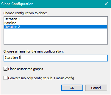
You'll be presented with the Clone Configuration dialog box. Select Iteration 2 in the Choose configuratio to clone list box, and enter Iteration 3 for the new configuration name. The dialog box should look like the figure below.

Click OK, then click on the Data View tab at the lower left of the MSO main window. It should look as follows:

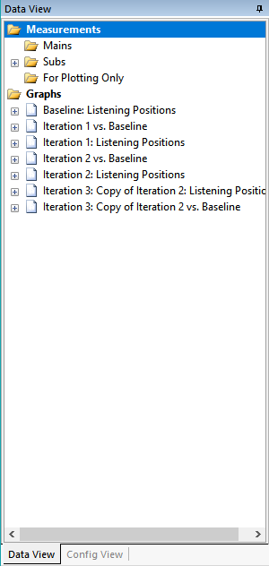
As with previous cloning steps, we ended up with some auto-generated graph names. They are:

Iteration 3: Copy of Iteration 2: Listening Positions
Iteration 3: Copy of Iteration 2 vs. Baseline

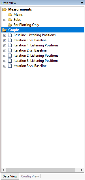
As before, we can rename these graphs by selecting them, pressing F2, and entering new text. Change their names to the following:

Iteration 3: Listening Positions
Iteration 3 vs. Baseline

The Data View should now look as below.

Data View After Renaming Iteration 3 Graphs

Select the Iteration 3 vs. Baseline graph, right-click on it, and choose Show Graph. This graph should look as below.

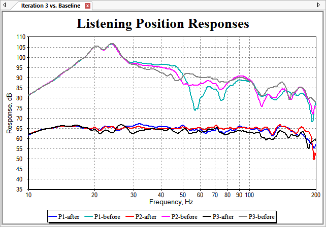
Graph of Newly-Cloned Iteration 3 vs. Baseline

Of course, this looks exactly like the corresponding plot of Iteration 2 vs. Baseline, since it is a clone and we haven't changed or added any filters yet.

Adding Shared Filters

Now we're ready to add some shared filters. We'll try six shared PEQs in this experiment. To add them, perform the following steps.

Select the Config View on the left side of the MSO main window.
Expand the Iteration 3 node.
Under Iteration 3, Filter Channels, Subwoofer Channels, Sub 1, Filters, select the filter FL1 and press Ctrl+C to copy it.
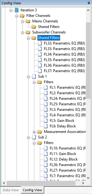
Select the Shared Filters node uder Iteration 3, Filter Channels, Subwoofer Channels. Press Ctrl+V six times to create six shared filters.

After performing these steps, we can see the new filters in the shared channel. This is shown below.

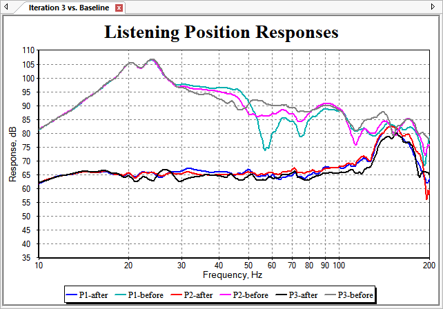
The Iteration 3 vs. Baseline graph has now changed, since we just pasted six PEQs into the shared filter channel. These PEQs all have the same parameter values and limits as FL1. The FL1 parameter values are not the default ones that result in a flat response for FL1, so the resulting response has some strange quirks. This doesn't matter, because we will set all the filter parameters back to their default values anyway before running an optimization. The Iteration 3 vs. Baseline graph now looks like the one below.

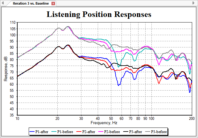
Graph of Iteration 3 vs. Baseline After Adding Shared Filters

Let's set all the filter parameters of Iteration 3 back to their default values. From the main menu, choose Config, Reset All Filter Parameter Values. Choose the Iteration 3 configuration and press OK. After making sure you actually chose Iteration 3 to reset, answer Yes to the prompt asking you if really want to reset the filters. After the reset, the Iteration 3 vs. Baseline graph should look like the figure below.

Graph of Iteration 3 vs. Baseline After Resetting All Filters

Let's do one final check to make sure our PEQ parameter limits are okay before optimizing. Right-click the Iteration 3 node in the Config View and choose Optimization Options. After the Optimization Options property sheet launches, choose PEQ Parameter Limits. This property page should appear as below.

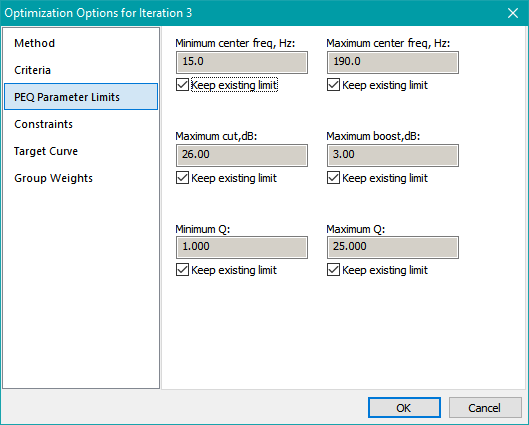
The trick of copying and pasting an existing filter into the shared filters worked. There is no mixture of different parameter limits, and they are all what we want them to be. That is, the PEQ center frequency limits are from 15 Hz to 190 Hz, their maximum cut is 26 dB, and their maximum boost is 3 dB. Click Cancel to dismiss the dialog.

Optimizing Iteration 3

Now we're ready to optimize the configuration. But before doing that, save the project as tutorial-new-5.msop. Then click the Run button on the toolbar to run the optimization. Make sure to choose Iteration 3 for the configuration to optimize.

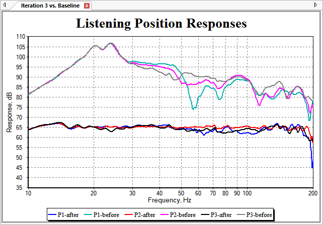
After running the optimization for 30 minutes on a machine supporting eight concurrent threads, the plot below was obtained. These results were saved in tutorial-new-6.msop.

Using the Configuration Performance Metrics Dialog to Compare Results

We can now use the Configuration Performance Metrics dialog to compare the errors of Iteration 1, Iteration 2 and Iteration 3. Choose Config, Performance Metrics from the main menu. For each of the configurations Iteration 1, Iteration 2 and Iteration 3, specify a custom frequency range, and set Minimum freq, Hz and Maximum freq, Hz to 15.0 Hz and 190.0 Hz respectively. If doing so activates the Recalculate button on any property page after making the change, click it to keep the calculations up to date. We obtain the results below.

Configuration	MLP target error	Seat-to-seat variation	Final error
Iteration 1	2.17 dB	1.31 dB	1.57 dB
Iteration 2	0.84 dB	0.79 dB	0.80 dB
Iteration 3	0.45 dB	0.72 dB	0.66 dB

Errors of Iteration 1, Iteration 2 and Iteration 3, 15 Hz - 190 Hz

Press Escape or click the Close button to dismiss the Configuration Performance Metrics dialog.

The data above show that Iteration 3 has given us a good improvement to the MLP response flatness, and a minor improvement to the seat-to-seat response variation when compared to Iteration 2. At first glance, it seems like this should be our final iteration.

Now is a good time to look at how to get the filter, delay and gain data into a DSP device. In the process of doing this in the next section, we'll run into a glitch and see how to resolve it.